Page 52 - Computational Colour Science Using MATLAB

IMPLEMENTATIONS AND EXAMPLES 39

function [cp] = cband2(p)

% applies Stearns-Stearns spectral bandpass correction
% operates on matrix P of dimensions n by m

a = 0.083;
dim = size(p);
n = dim(1);

for i = 2:n-1
cp(i,:) = -a*p(i-1,:) + (1 + 2*a)*p(i,:) - a*p(i+1,:);
end
cp(1,:) = (1 + a)*p(1,:) - a*p(2,:);
cp(n,:) = (1 + a)*p(n,:) - a*p(n-1,:);

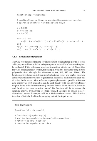
4.8.2 Reflectance interpolation

The CIE recommended method for interpolation of reflectance spectra is to use
cubic polynomial interpolation using two points either side of the wavelength to
be evaluated. If the reflectance spectrum is available at intervals of 20 nm, then
the value of reflectance at 470 nm, for example, would be calculated using a cubic
polynomial fitted through the reflectance at 440, 460, 480 and 500 nm. The
function pinterp takes an N-dimensional reflectance vector and applies piecewise
cubic polynomial interpolation to generate an additional point between each pair
of points in the vector. Most reflectance spectrophotometers provide reflectance
data at intervals of 10 nm and so can be used directly with the ASTM tables of
weights. Some older instruments only produce data at 20-nm intervals, however,
and therefore the most practical use of this function will be to reduce the
sampling interval from 20 nm to 10 nm. Thus, if the input to pinterp is a 16-
dimensional vector the output will be a 31-dimensional vector. This function
therefore effectively doubles the sampling rate of the input vector.

Box 2: pinterp.m

function [s] = pinterp(p)

% function [s] = pinterp(p)
% applies interpolation to double the sampling
% rate of the n by 1 matrix p
% returns interpolated matrix s