Page 112 - Computational Modeling in Biomedical Engineering and Medical Physics
P. 112

Electrical activity of the heart  101


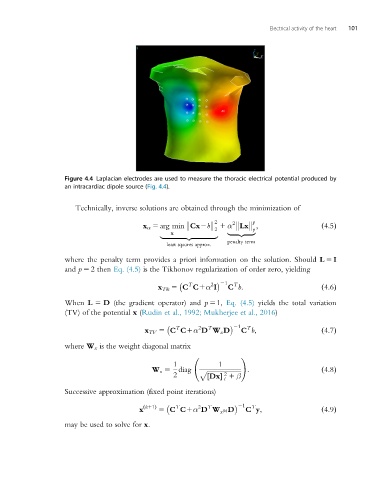
                   Figure 4.4 Laplacian electrodes are used to measure the thoracic electrical potential produced by
                   an intracardiac dipole source (Fig. 4.4).


                      Technically, inverse solutions are obtained through the minimization of
                                                            2    2     p
                                         x α 5 arg min :Cx2b: 1 α :Lx: ;                  ð4:5Þ
                                                                       p
                                                            2
                                                x
                                                                |fflfflfflfflffl{zfflfflfflfflffl}
                                             |fflfflfflfflfflfflfflfflfflfflfflfflfflffl{zfflfflfflfflfflfflfflfflfflfflfflfflfflffl}
                                                                penalty term
                                               least sqaures approx:
                   where the penalty term provides a priori information on the solution. Should L 5 I
                   and p 5 2 then Eq. (4.5) is the Tikhonov regularization of order zero, yielding
                                                      T    2    21  T
                                             x Tik 5 C C1α I    C b:                      ð4:6Þ
                   When L 5 D (the gradient operator) and p 51, Eq. (4.5) yields the total variation
                   (TV) of the potential x (Rudin et al., 1992; Mukherjee et al., 2016)
                                                  T
                                                        2
                                         x TV 5 C C1α D W x D      21 C b;                ð4:7Þ
                                                                     T

                                                           T
                   where W x is the weight diagonal matrix
                                                                    !
                                                 1            1
                                           W x 5 diag   p ffiffiffiffiffiffiffiffiffiffiffiffiffiffiffiffiffiffiffiffiffi :         ð4:8Þ
                                                 2         DxŠ 1 β
                                                               2
                                                          ½    i
                   Successive approximation (fixed point iterations)
                                        x ðk11Þ 5 C C1α D W ðkÞD    21 C y;               ð4:9Þ
                                                                       T

                                                  T
                                                           T
                                                        2
                                                              x
                   may be used to solve for x.
   107   108   109   110   111   112   113   114   115   116   117