Page 211 - Computational Retinal Image Analysis

2 Structure-preserving guided retinal image filtering 207

pixels. The averaging in the above process often smooths away the fine structure
in regions close to flat-costrast ones, which is not optimal for retinal images: for
example, the boundaries between the optic cup and the neuroretinal rim can be
weak in some cases. The averaging in such regions might smooth away the weak
boundaries and make the segmentation of optic cup more challenging.
To address this problem, we propose a novel structure-preserving guided retinal
image filter (SGRIF). Inspired by GIF [53], we aim to transfer the structure of G to I to
preserve the edges and smooth the transferred image. The proposed SGRIF is composed
of a global structure transfer filter to transfer the structure in the retinal image and a
global edge-preserving smoothing filter to smooth the transferred retinal image. To
h
v
achieve that, we need to compute a guidance vector field V = (V , V ). The inputs of the
proposed SGRIF are a retinal image and the vector V. A term computing the difference
of the gradients of the output image O and the vector V is computed to penalize the
transfer:

∑∇O −V  2 , (10)
i i i
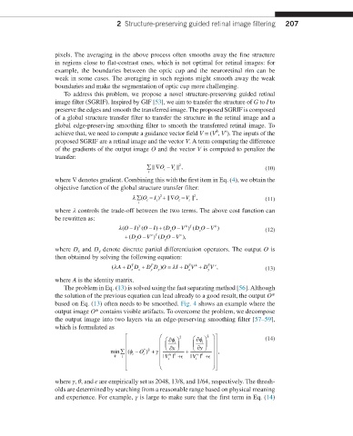
where ∇ denotes gradient. Combining this with the first item in Eq. (4), we obtain the
objective function of the global structure transfer filter:

λ ∑ O − I ) 2 +∇O −V  2 , (11)
(
i i i i i
where λ controls the trade-off between the two terms. The above cost function can
be rewritten as:
−
T
−
−
+
) (D OV
λ(OI ) (OI ) (DO V hT − h )
x x (12)
+ (DO V vT y − v ),
−
) (D OV
y
where D x and D y denote discrete partial differentiation operators. The output O is
then obtained by solving the following equation:
T
) =
h
+
T
(λAD D + D DO λI + D V + D V v , (13)
T
T
y
y
y
x
x
x
where A is the identity matrix.
The problem in Eq. (13) is solved using the fast separating method [56]. Although
the solution of the previous equation can lead already to a good result, the output O*
based on Eq. (13) often needs to be smoothed. Fig. 4 shows an example where the
output image O* contains visible artifacts. To overcome the problem, we decompose
the output image into two layers via an edge-preserving smoothing filter [57–59],
which is formulated as
    ∂ φ  2  ∂ φ  2  (14)
   i   i  
y
∂ 
min∑   (φ − O * 2 γ    x +  ∂   ,
) +

φ i i i |V h | + θ |V v | + θ
  i i 
  
  
where γ, θ, and ϵ are empirically set as 2048, 13/8, and 1/64, respectively. The thresh-
olds are determined by searching from a reasonable range based on physical meaning
and experience. For example, γ is large to make sure that the first term in Eq. (14)