Page 212 - Computational Retinal Image Analysis

208 CHAPTER 11 Structure-preserving guided retinal image filtering

(A) (B) (C)
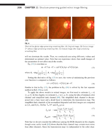
FIG. 4
Effect of the global edge-preserving smoothing filter. (A) Original image. (B) Output image
O* without edge-preserving smoothing filter. (C) Output image after edge-preserving
smoothing filter.

will not dominate the results. Then, we conducted tests using different γ values and
determined an optimal value. Note that our experience shows that small changes of
the parameters do not affect much the results.
Eq. (14) is rewritten as
+
+
T
T
T
T
(
) (φ − O
(φ − O * T * ) γφ DB D x φφ D BD y φ ), (15)
y
y
x
x
  1     1  
where B = diag  h θ  , B = diag  v θ  .
y
x


  V | i | +    V | i | +  

Setting the derivative of Eq. (15) to zero, the vector ϕ minimizing the previous
cost function is computed as follows:
φ
T
T
(A + γ (D BD + DB D y )) = O * . (16)
y
x
y
x
x
Similar to that in Eq. (13), the problem in Eq. (16) is solved by the fast separate
method in Ref. [56] as well.
To apply the above models to retinal images, we first need to estimate L c , c ∈
{r, g, b}. In this chapter, we estimate L c , c ∈{r, g, b}, using the idea of minimal color
channel and simplified dark channel [60]. The simplified dark channel is decom-
posed into a base layer and a detail layer to determine the transmission map. The
simplified dark channels of the normalized degraded and ideal images are computed

as I c /L c and D c /L c . Define I  min p () and D () as
p
min
  Ip Ip Ip()  (17)
()
()

I  min p () = min  r , g , b , 
  L r L g L b  
  Dp Dp Dp() 
()

()

D () = min  r , g , b .  (18)
p
min
  L r L g L b  
Note that we do not consider the difference among the RGB channels in this chapter,
though some earlier work [61] shows that the blue channel may contain more noise
than other channels. Since the transmission map t is independent to the color chan-