Page 217 - Computational Retinal Image Analysis

3 Experimental results 213

segmentation. In our implementation, we use a simplified U-Net as it requires fewer
parameters to be trained compared with the original U-Net. As shown in Fig. 6, our
network contains an encoder and a decoder similar to the original U-Net. For each
layer in the encoder, it just adopts a convolution layer with stride 2, replacing the
original two convolution layers and one pooling layer. For each layer in the decoder,
it takes two inputs: (i) the output of last layer in the encoder; (ii) the corresponding
layer in the encoder with the same size. Then, two middle-layer feature maps are
concatenated and transferred to the next deconvolution layer as its input. Finally,
our simplified U-Net outputs a prediction grayscale map, which ranges from 0 to
255. We calculate the mean square error between prediction map and ground truth as
loss function. In our simple U-Net, we use a mini-batch stochastic gradient decent
(SGD) algorithm to optimize the loss function, specifically, Adagrad-based SGD
[67]. The adopted learning rate is 0.001 and the batch size is 32 under the Tensorflow
framework based on Ubuntu 16.04 system. We use a momentum of 0.9. All images
are resized to 384 × 384 for training and testing. The obtained probability map is
resized back to original size to obtain the segmentation results.
In our experiments, the 650 images have been divided randomly into set A of 325
training images and set B of 325 testing images. To evaluate the performance of the
algorithm in the presence of cataracts, the 325 images in set B are further divided into a
subset of 113 images with cataracts and 212 images without cataract. We then compare
the results in the following three different scenarios: (1) Original: the original training
and testing images are used for training and testing the U-Net model; (2) GIF: all
images are first processed by GIF before U-Net model training and testing; (3) SGRIF:
all images are first filtered by SGRIF before U-Net model training and testing.
The commonly used overlapping error E is computed as the evaluation metric.
Area S ∩( G)
E =− , (30)
1
Area S ∪( G)
where S and G denote the segmented and the manual “ground truth” optic cup, re-
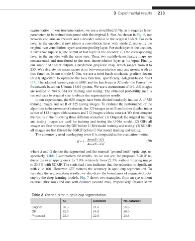
spectively. Table 2 summarizes the results. As we can see, the proposed SGRIF re-
duces the overlapping error by 7.9% relatively from 25.3% without filtering image
to 23.3% with SGRIF. The statistical t-test indicates that the reduction is significant
with P < .001. However, GIF reduces the accuracy in optic cup segmentation. To
visualize the segmentation results, we also draw the boundaries of segmented optic
cup by the deep learning models. Fig. 7 shows two examples, from an eye without
cataract (first row) and one with cataract (second row), respectively. Results show

Table 2 Overlap error in optic cup segmentation.
All Cataract No cataract
Original 25.3 24.4 25.8
GIF 25.6 24.8 26.0
Proposed 23.3 22.8 23.5