Page 218 - Computational Retinal Image Analysis

214 CHAPTER 11 Structure-preserving guided retinal image filtering

(A) (B) (C) (D) (E)
FIG. 7
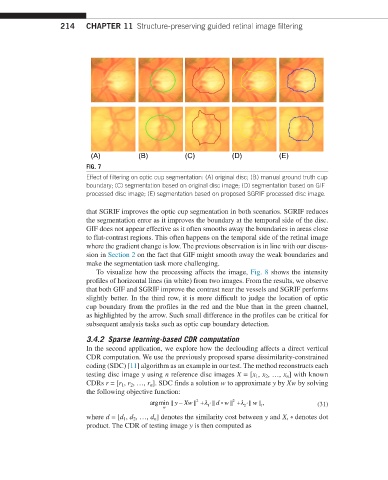
Effect of filtering on optic cup segmentation: (A) original disc; (B) manual ground truth cup
boundary; (C) segmentation based on original disc image; (D) segmentation based on GIF
processed disc image; (E) segmentation based on proposed SGRIF processed disc image.

that SGRIF improves the optic cup segmentation in both scenarios. SGRIF reduces
the segmentation error as it improves the boundary at the temporal side of the disc.
GIF does not appear effective as it often smooths away the boundaries in areas close
to flat-contrast regions. This often happens on the temporal side of the retinal image
where the gradient change is low. The previous observation is in line with our discus-
sion in Section 2 on the fact that GIF might smooth away the weak boundaries and
make the segmentation task more challenging.
To visualize how the processing affects the image, Fig. 8 shows the intensity
profiles of horizontal lines (in white) from two images. From the results, we observe
that both GIF and SGRIF improve the contrast near the vessels and SGRIF performs
slightly better. In the third row, it is more difficult to judge the location of optic
cup boundary from the profiles in the red and the blue than in the green channel,
as highlighted by the arrow. Such small difference in the profiles can be critical for
subsequent analysis tasks such as optic cup boundary detection.
3.4.2 Sparse learning-based CDR computation
In the second application, we explore how the declouding affects a direct vertical
CDR computation. We use the previously proposed sparse dissimilarity-constrained
coding (SDC) [11] algorithm as an example in our test. The method reconstructs each
testing disc image y using n reference disc images X = [x 1 , x 2 , …, x n ] with known
CDRs r = [r 1 , r 2 , …, r n ]. SDC finds a solution w to approximate y by Xw by solving
the following objective function:

2
λ
d w + ⋅
argmin y − Xw + ⋅ 2 λ w , (31)
w 1 2 1
where d = [d 1 , d 2 , …, d n ] denotes the similarity cost between y and X, ∘ denotes dot
product. The CDR of testing image y is then computed as