Page 105 - Computational Statistics Handbook with MATLAB

92 Computational Statistics Handbook with MATLAB

λx – y t – 1
e y
Fx() = ∫ -----------------d . y (4.12)
(
1)!
t –
0
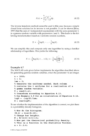
The inverse transform method cannot be used in this case, because a simple
closed form solution for its inverse is not possible. It can be shown [Ross,
1997] that the sum of t independent exponentials with the same parameter λ
λ
is a gamma random variable with parameters t and . This leads to the fol-
lowing transformation based on t uniform random numbers,

1 1
X = – ---log U 1 – … – ---log U t . (4.13)
λ λ
We can simplify this and compute only one logarithm by using a familiar
relationship of logarithms. This yields the following

1 1  t 
X = – ---log ( U 1 × … × U t ) = – ---log  ∏ U i .  (4.14)
λ λ  
i = 1

Example 4.7
The MATLAB code given below implements the algorithm described above
for generating gamma random variables, when the parameter t is an integer.
n = 1000;
t = 3;
lam = 2;
% Generate the uniforms needed. Each column
% contains the t uniforms for a realization of a
% gamma random variable.
U = rand(t,n);
% Transform according to Equation 4.13.
% See Example 4.8 for an illustration of Equation 4.14.
logU = -log(U)/lam;
X = sum(logU);

To see whether the implementation of the algorithm is correct, we plot them
in a probability density histogram.
% Now do the histogram.
[N,h] = hist(X,10);
% Change bar heights.
N = N/(h(2)-h(1))/n;
% Now get the theoretical probability density.
% This is a function in the Statistics Toolbox.
x = 0:.1:6;

© 2002 by Chapman & Hall/CRC