Page 110 - Computational Statistics Handbook with MATLAB

Chapter 4: Generating Random Variables 97

α = β = 3 α = β = 0.5
2.5 3.5

3
2
2.5
1.5
2

1.5
1
1
0.5
0.5

0 0
0 0.5 1 0 0.5 1
U
F FI IG URE G 4. RE 4. 6 6
F F II GU RE RE 4. 4. 6
GU
6
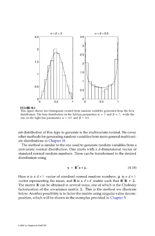
This figure shows two histograms created from random variables generated from the beta
distribution. The beta distribution on the left has parameters α = 3 and β = 3, while the
one on the right has parameters α = 0.5 and β = 0.5.
est distribution of this type to generate is the multivariate normal. We cover
other methods for generating random variables from more general multivari-
ate distributions in Chapter 11.
The method is similar to the one used to generate random variables from a
univariate normal distribution. One starts with a d-dimensional vector of
standard normal random numbers. These can be transformed to the desired
distribution using

T
x = R z + µ . (4.18)

µ µ µ µ
Here z is a d × 1 vector of standard normal random numbers, is a d × 1
T
vector representing the mean, and R is a d × d matrix such that R R = Σ.
The matrix R can be obtained in several ways, one of which is the Cholesky
factorization of the covariance matrix Σ. This is the method we illustrate
below. Another possibility is to factor the matrix using singular value decom-
position, which will be shown in the examples provided in Chapter 5.

© 2002 by Chapman & Hall/CRC