Page 344 - Computational Statistics Handbook with MATLAB

Chapter 9: Statistical Pattern Recognition 333

e
eenntt
e
eependpend
est
ple
ple
TS Sa
amm
Ind ependpend ennt tT TTestest est SS aamm pleple
IndInd
Ind
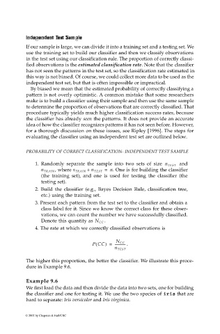
If our sample is large, we can divide it into a training set and a testing set. We
use the training set to build our classifier and then we classify observations
in the test set using our classification rule. The proportion of correctly classi-
fied observations is the estimated classification rate. Note that the classifier
has not seen the patterns in the test set, so the classification rate estimated in
this way is not biased. Of course, we could collect more data to be used as the
independent test set, but that is often impossible or impractical.
By biased we mean that the estimated probability of correctly classifying a
pattern is not overly optimistic. A common mistake that some researchers
make is to build a classifier using their sample and then use the same sample
to determine the proportion of observations that are correctly classified. That
procedure typically yields much higher classification success rates, because
the classifier has already seen the patterns. It does not provide an accurate
idea of how the classifier recognizes patterns it has not seen before. However,
for a thorough discussion on these issues, see Ripley [1996]. The steps for
evaluating the classifier using an independent test set are outlined below.
PROBABILITY OF CORRECT CLASSIFICATION- INDEPENDENT TEST SAMPLE
and
1. Randomly separate the sample into two sets of size n TEST
, where n TRAIN + n TEST = n . One is for building the classifier
n TRAIN
(the training set), and one is used for testing the classifier (the
testing set).
2. Build the classifier (e.g., Bayes Decision Rule, classification tree,
etc.) using the training set.
3. Present each pattern from the test set to the classifier and obtain a
class label for it. Since we know the correct class for these obser-
vations, we can count the number we have successfully classified.
.
Denote this quantity as N CC
4. The rate at which we correctly classified observations is

(
N CC
PCC) = ------------- .
n TEST
The higher this proportion, the better the classifier. We illustrate this proce-
dure in Example 9.6.

Example 9.6
We first load the data and then divide the data into two sets, one for building
the classifier and one for testing it. We use the two species of iris that are
hard to separate: Iris versicolor and Iris virginica.

© 2002 by Chapman & Hall/CRC