Page 342 - Computational Statistics Handbook with MATLAB

Chapter 9: Statistical Pattern Recognition 331

0.25
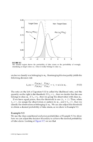
Target Class Non−Target Class

0.2
P(x | ω )*P(ω ) P(x | ω )*P(ω )
1 1 2 2
0.15

0.1

0.05

0
−6 −4 −2 0 2 4 6 8

U
FI F IG URE G 9. RE 9. 7 7
7
GU
F F II GU RE RE 9. 9. 7
The shaded region shows the probability of false alarm or the probability of wrongly
) when it really belongs to class ω 2 .
classifying as target (class ω 1
or else we classify x as belonging to ω 2 . Rearranging this inequality yields the
following decision rule
P x ω 1 ) P ω 2 )
(
(
L R x() = -------------------- > --------------- = τ C ⇒ x is in ω 1 . (9.10)
(
(
P x ω 2 ) P ω 1 )
The ratio on the left of Equation 9.10 is called the likelihood ratio, and the
quantity on the right is the threshold. If L > τ C , then we decide that the case
R
belongs to class ω 1 . If L < τ C , then we group the observation with class ω 2 .
R
If we have equal priors, then the threshold is one (τ = 1 ). Thus, when
C
L > 1 , we assign the observation or pattern to ω 1 , and if L < 1 , then we
R
R
classify the observation as belonging to ω 2 . We can also adjust this threshold
to obtain a desired probability of false alarm, as we show in Example 9.5.
Example 9.5
We use the class-conditional and prior probabilities of Example 9.3 to show
how we can adjust the decision boundary to achieve the desired probability
of false alarm. Looking at Figure 9.7, we see that

© 2002 by Chapman & Hall/CRC