Page 338 - Computational Statistics Handbook with MATLAB

Chapter 9: Statistical Pattern Recognition 327

0.25

0.2

0.15

0.1

0.05

0
−6 −4 −2 0 2 4 6 8
Feature − x

U
FI F IG URE G 9. RE 9. 4 4
F F II GU RE RE 9. 9. 4
GU
4
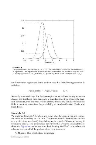
The vertical dotted line represents x = – 0.75 . The probabilities needed for the decision rule
of Equation 9.7 are represented by the horizontal dotted lines. We would classify this case
).
as belonging to class 1 ( ω 1 ), but there is a possibility that it could belong to class 2 ( ω 2
for the decision regions are found as the x such that the following equation is
satisfied:
P x ω )P ω( ) = P x ω )P ω ); i ≠ . j
(
(
(
j j i i
Secondly, we can change this decision region as we will see shortly when we
discuss the likelihood ratio approach to classification. If we change the deci-
sion boundary, then the error will be greater, illustrating that Bayes Decision
Rule is one that minimizes the probability of misclassification [Duda and
Hart, 1973].

Example 9.4
We continue Example 9.3, where we show what happens when we change
the decision boundary to x = – 0.5 . This means that if a feature has a value
of x < – 0.5 , then we classify it as belonging to class 1. Otherwise, we say it
belongs to class 2. The areas under the curves that we need to calculate are
shown in Figure 9.6. As we see from the following MATLAB code, where we
estimate the error, that the probability of error increases.
% Change the decision boundary.
© 2002 by Chapman & Hall/CRC