Page 337 - Computational Statistics Handbook with MATLAB

326 Computational Statistics Handbook with MATLAB

0.25

P(x | ω ) * P(ω )
0.2 P(x | ω ) * P(ω ) 2 2
1 1

0.15

0.1

0.05

0
−6 −4 −2 0 2 4 6 8
Feature − x

U
F FI IG URE G 9. RE 9. 3 3
F F II GU RE RE 9. 9. 3
GU
3
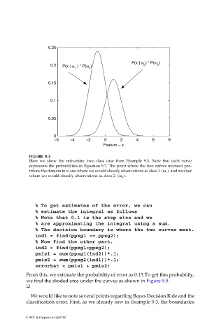
Here we show the univariate, two class case from Example 9.3. Note that each curve
represents the probabilities in Equation 9.7. The point where the two curves intersect par-
titions the domain into one where we would classify observations as class 1 ω 1 ) and another
(
(
where we would classify observations as class 2 ω 2 ).
% To get estimates of the error, we can
% estimate the integral as follows
% Note that 0.1 is the step size and we
% are approximating the integral using a sum.
% The decision boundary is where the two curves meet.
ind1 = find(ppxg1 >= ppxg2);
% Now find the other part.
ind2 = find(ppxg1<ppxg2);
pmis1 = sum(ppxg1(ind2))*.1;
pmis2 = sum(ppxg2(ind1))*.1;
errorhat = pmis1 + pmis2;
From this, we estimate the probability of error as 0.15. To get this probability,
we find the shaded area under the curves as shown in Figure 9.5.

We would like to note several points regarding Bayes Decision Rule and the
classification error. First, as we already saw in Example 9.3, the boundaries

© 2002 by Chapman & Hall/CRC