Page 336 - Computational Statistics Handbook with MATLAB

Chapter 9: Statistical Pattern Recognition 325

(
(
,
Px ω ) = φ x; – 11)
1
(
(
,
Px ω 2 ) = φ x 11).
;
The priors are
(
P ω 1 ) = 0.6
(
P ω 2 ) = 0.4.
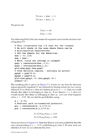
The following MATLAB code creates the required curves for the decision rule
of Equation 9.7.
% This illustrates the 1-D case for two classes.
% We will shade in the area where there can be
% misclassified observations.
% Get the domain for the densities.
dom = -6:.1:8;
dom = dom';
% Note: could use csnormp or normpdf.
pxg1 = csevalnorm(dom,-1,1);
pxg2 = csevalnorm(dom,1,1);
plot(dom,pxg1,dom,pxg2)
% Find decision regions - multiply by priors
ppxg1 = pxg1*0.6;
ppxg2 = pxg2*0.4;
plot(dom,ppxg1,'k',dom,ppxg2,'k')
xlabel('x')
The resulting plot is given in Figure 9.3, where we see that the decision
regions given by Equation 9.7 are obtained by finding where the two curves
intersect. If we observe a value of a feature given by x = – 2 , then we would
. If we observe x = 4 , then we
classify that object as belonging to class ω 1
. Let’s see what happens
would classify that object as belonging to class ω 2
when x = – 0.75 . We can find the probabilities using
x = -0.75;
% Evaluate each un-normalizd posterior.
po1 = csevalnorm(x,-1,1)*0.6;
po2 = csevalnorm(x,1,1)*0.4;

P – ( 0.75 ω )P ω( ) = 0.23
1 1
P – ( 0.75 ω 2 )P ω 2 ) = 0.04.
(
These are shown in Figure 9.4. Note that there is non-zero probability that the
case corresponding to x = – 0.75 could belong to class 2. We now turn our
attention to how we can estimate this error.
© 2002 by Chapman & Hall/CRC