Page 305 -

Section 9.3 Image Segmentation by Clustering Pixels 273

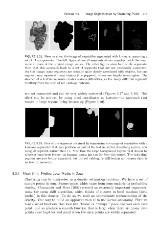
FIGURE 9.18: Here we show the image of vegetables segmented with k-means, assuming a
set of 11 components. The left figure shows all segments shown together, with the mean
value in place of the original image values. The other figures show four of the segments.
Note that this approach leads to a set of segments that are not necessarily connected.
For this image, some segments are actually quite closely associated with objects, but one
segment may represent many objects (the peppers); others are largely meaningless. The
absence of a texture measure creates serious difficulties, as the many different segments
resulting from the slice of red cabbage indicate.

are not connected and can be very widely scattered (Figures 9.17 and 9.18). This
effect can be reduced by using pixel coordinates as features—an approach that
results in large regions being broken up (Figure 9.19).

FIGURE 9.19: Five of the segments obtained by segmenting the image of vegetables with a
k-means segmenter that uses position as part of the feature vector describing a pixel, now
using 20 segments rather than 11. Note that the large background regions that should be
coherent have been broken up because points got too far from the center. The individual
peppers are now better separated, but the red cabbage is still broken up because there is
no texture measure.

9.3.4 Mean Shift: Finding Local Modes in Data

Clustering can be abstracted as a density estimation problem. We have a set of
sample points in some feature space, which came from some underlying probability
density. Comaniciu and Meer (2002) created an extremely important segmenter,
using the mean shift algorithm, which thinks of clusters as local maxima (local
modes) in this density. To do so, we need an approximate representation of the
density. One way to build an approximation is to use kernel smoothing.Here we
take a set of functions that look like “blobs” or “bumps,” place one over each data
point, and so produce a smooth function that is large when there are many data
points close together and small when the data points are widely separated.