Page 306 -

Section 9.3 Image Segmentation by Clustering Pixels 274

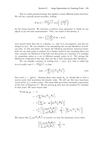
This is a quite general strategy that applies to many different bump functions.
We will use a specific kernel smoother, writing

2
(2π) (−d/2) 1 ||x||
K(x; h)= exp −
h d 2 h
for the bump function. We introduce a positive scale parameter h, which we can
adjust to get the best representation. Then, our model of the density is

n
1
f(x)= K (x i − x; h)
n
i=1
(you should check that this is a density, i.e., that it is non-negative, and that its
integral is one). We can estimate h by maximizing the average likelihood of held-
out data. In this procedure, we repeat the following experiment numerous times:
hold out one data point at random, fit a density model to the remaining data, and
then compute the likelihood of the held-out data point as a function of h (perhaps
by computing values at a set of different sample points in h). We average the
likelihoods computed in this way, then use the h that maximizes that likelihood.

1
We can simplify notation by writing k(u)=exp − u (this is called the
2
(2π) (−d/2)
kernel profile)and C = ,so that
nh d
n
x − x i 2
f(x)= C k || || (9.1)
h
i=1
Now write g = d k(u). Starting from some point x 0 , we should like to find a
du
nearby point that maximizes the density value. We will use this local maximum
(local mode) as a cluster center. The mean shift procedure maximizes expressions
of the form of Equation 9.1. We are seeking y such that the gradient ∇f vanishes
at that point. We must require that

∇f(x) |x=y = 0
x i − y
2
= C ∇k(|| || )
h
i
- 2 .
2 x i − y
= C [x i − y] g(|| || )
h h
i
# $ # $
x i −y 2
2 i x i g(|| h || ) x i − y 2
= C 2 − y × g(|| || ) .
h x i −y h
i g(|| h || ) i
x i −y 2
We expect that g(|| || ) is nonzero, so that the maximum occurs when
i h
# $
x i −y 2
x i g(|| || )
i h − y =0,
x i −y 2
i g(|| h || )