Page 335 -

Section 10.4 Robustness 303

6 6 6
4 4 4
2 2 2
0 0 0
-2 -2 -2
-4 -4 -4
-6 -6 -6
-8 -8 -8
-10 -10 -10
-12 -12 -12
-14 -14 -14
-14 -12 -10 -8 -6 -4 -2 0 2 4 6 -14 -12 -10 -8 -6 -4 -2 0 2 4 6 -14 -12 -10 -8 -6 -4 -2 0 2 4 6
2 2 2
1.5 1.5 1.5
1 1 1
0.5 0.5 0.5
0 0 0
-0.5 -0.5 -0.5
-1 -1 -1
-1.5 -1.5 -1.5
-2 -2 -2
-2 -1.5 -1 -0.5 0 0.5 1 1.5 2 -2 -1.5 -1 -0.5 0 0.5 1 1.5 2 -2 -1.5 -1 -0.5 0 0.5 1 1.5 2
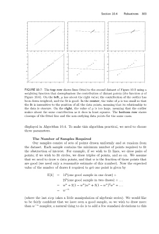
FIGURE 10.7: The top row shows lines fitted to the second dataset of Figure 10.5 using a
weighting function that deemphasizes the contribution of distant points (the function φ of
Figure 10.6). On the left, μ has about the right value; the contribution of the outlier has
been down-weighted, and the fit is good. In the center,the value of μ is too small so that
the fit is insensitive to the position of all the data points, meaning that its relationship to
the data is obscure. On the right,the value of μ is too large, meaning that the outlier
makes about the same contribution as it does in least squares. The bottom row shows
closeups of the fitted line and the non-outlying data points for the same cases.

displayed in Algorithm 10.4. To make this algorithm practical, we need to choose
three parameters.

The Number of Samples Required
Our samples consist of sets of points drawn uniformly and at random from
the dataset. Each sample contains the minimum number of points required to fit
the abstraction of interest. For example, if we wish to fit lines, we draw pairs of
points; if we wish to fit circles, we draw triples of points, and so on. We assume
that we need to draw n data points, and that w is the fraction of these points that
are good (we need only a reasonable estimate of this number). Now the expected
value of the number of draws k required to get one point is given by
E[k]= 1P(one good sample in one draw) +
2P(one good sample in two draws) + ...
n
n
n
n 2
n
= w +2(1 − w )w +3(1 − w ) w + ...
= w −n
(where the last step takes a little manipulation of algebraic series). We would like
to be fairly confident that we have seen a good sample, so we wish to draw more
than w −n samples; a natural thing to do is to add a few standard deviations to this