Page 330 -

Section 10.3 Fitting Curved Structures 298

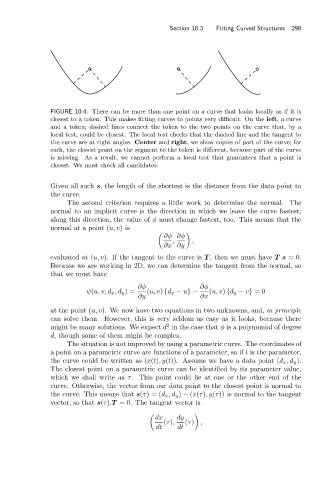
FIGURE 10.4: There can be more than one point on a curve that looks locally as if it is
closest to a token. This makes fitting curves to points very difficult. On the left, a curve
and a token; dashed lines connect the token to the two points on the curve that, by a
local test, could be closest. The local test checks that the dashed line and the tangent to
the curve are at right angles. Center and right, we show copies of part of the curve; for
each, the closest point on the segment to the token is different, because part of the curve
is missing. As a result, we cannot perform a local test that guarantees that a point is
closest. We must check all candidates.

Given all such s, the length of the shortest is the distance from the data point to
the curve.
The second criterion requires a little work to determine the normal. The
normal to an implicit curve is the direction in which we leave the curve fastest;
along this direction, the value of φ must change fastest, too. This means that the
normal at a point (u, v)is

∂φ ∂φ
, ,
∂x ∂y
evaluated at (u, v). If the tangent to the curve is T , then we must have T .s =0.
Because we are working in 2D, we can determine the tangent from the normal, so
that we must have
∂φ ∂φ
ψ(u, v; d x ,d y )= (u, v) {d x − u}− (u, v) {d y − v} =0
∂y ∂x

at the point (u, v). We now have two equations in two unknowns, and, in principle
can solve them. However, this is very seldom as easy as it looks, because there
2
might be many solutions. We expect d in the case that φ is a polynomial of degree
d, though some of them might be complex.
The situation is not improved by using a parametric curve. The coordinates of
a point on a parametric curve are functions of a parameter, so if t is the parameter,
the curve could be written as (x(t),y(t)). Assume we have a data point (d x ,d y ).
The closest point on a parametric curve can be identified by its parameter value,
which we shall write as τ. This point could lie at one or the other end of the
curve. Otherwise, the vector from our data point to the closest point is normal to
the curve. This means that s(τ)= (d x ,d y ) − (x(τ),y(τ)) is normal to the tangent
vector, so that s(τ).T = 0. The tangent vector is

dx dy
(τ), (τ) ,
dt dt