Page 327 -

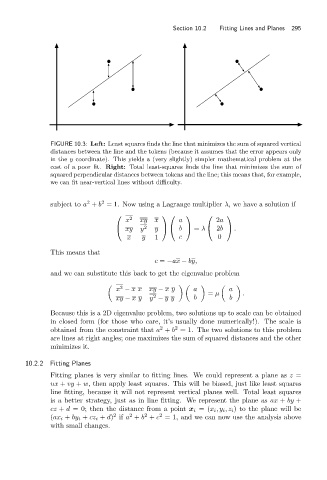
Section 10.2 Fitting Lines and Planes 295

FIGURE 10.3: Left: Least squares finds the line that minimizes the sum of squared vertical
distances between the line and the tokens (because it assumes that the error appears only
in the y coordinate). This yields a (very slightly) simpler mathematical problem at the
cost of a poor fit. Right: Total least-squares finds the line that minimizes the sum of
squared perpendicular distances between tokens and the line; this means that, for example,
we can fit near-vertical lines without difficulty.

2
2
subject to a + b = 1. Now using a Lagrange multiplier λ, we have a solution if
⎛ ⎞ ⎛ ⎞ ⎛ ⎞
x 2 xy x a 2a
xy y y
⎝ 2 ⎠ ⎝ b ⎠ = λ ⎝ 2b ⎠ .
x y 1 c 0
This means that
c = −ax − by,
and we can substitute this back to get the eigenvalue problem

2
x − x x xy − x y a a
= μ .
2
xy − x y y − y y b b
Because this is a 2D eigenvalue problem, two solutions up to scale can be obtained
in closed form (for those who care, it’s usually done numerically!). The scale is
2
2
obtained from the constraint that a + b = 1. The two solutions to this problem
are lines at right angles; one maximizes the sum of squared distances and the other
minimizes it.
10.2.2 Fitting Planes
Fitting planes is very similar to fitting lines. We could represent a plane as z =
ux + vy + w, then apply least squares. This will be biased, just like least squares
line fitting, because it will not represent vertical planes well. Total least squares
is a better strategy, just as in line fitting. We represent the plane as ax + by +
cz + d = 0; then the distance from a point x i =(x i ,y i ,z i ) to the plane will be
2
2
2
2
(ax i + by i + cz i + d) if a + b + c = 1, and we can now use the analysis above
with small changes.