Page 332 -

Section 10.4 Robustness 300

6 6
4 4
2 2
0 0
-2 -2
-4 -4
-6 -6
-8 -8
-10 -10
-12 -12
-14 -14
-14 -12 -10 -8 -6 -4 -2 0 2 4 6 -14 -12 -10 -8 -6 -4 -2 0 2 4 6
2
6
4 1.5
2
1
0
0.5
-2
0
-4
-6
-0.5
-8
-1
-10
-1.5
-12
-14 -2
-14 -12 -10 -8 -6 -4 -2 0 2 4 6 -2 -1.5 -1 -0.5 0 0.5 1 1.5 2
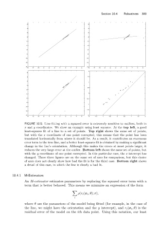
FIGURE 10.5: Line fitting with a squared error is extremely sensitive to outliers, both in
x and y coordinates. We show an example using least squares. At the top left, a good
least-squares fit of a line to a set of points. Top right shows the same set of points,
but with the x coordinate of one point corrupted; this means that the point has been
translated horizontally from where it should be. As a result, it contributes an enormous
error term to the true line, and a better least-squares fit is obtained by making a significant
change in the line’s orientation. Although this makes the errors at most points larger, it
reduces the very large error at the outlier. Bottom left shows the same set of points, but
with the y coordinate of one point corrupted. In this particular case, the x intercept has
changed. These three figures are on the same set of axes for comparison, but this choice
of axes does not clearly show how bad the fit is for the third case. Bottom right shows
a detail of this case, in which the line is clearly a bad fit.

10.4.1 M-Estimators
An M-estimator estimates parameters by replacing the squared error term with a
term that is better behaved. This means we minimize an expression of the form

ρ(r i (x i ,θ); σ),
i
where θ are the parameters of the model being fitted (for example, in the case of
the line, we might have the orientation and the y intercept), and r i (x i ,θ)is the
residual error of the model on the ith data point. Using this notation, our least