Page 333 -

Section 10.4 Robustness 301

2
1.8
1.6
2
y=x
1.4
1.2
1
0.1
0.8
1
0.6
10
0.4
0.2
0
-10 -8 -6 -4 -2 0 2 4 6 8 10
2
2
2
2
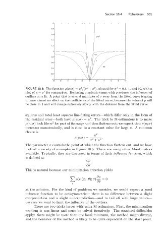
FIGURE 10.6: The function ρ(x; σ)= x /(σ + x ), plotted for σ =0.1, 1, and 10, with a
2
plot of y = x for comparison. Replacing quadratic terms with ρ reduces the influence of
outliers on a fit. A point that is several multiples of σ away from the fitted curve is going
to have almost no effect on the coefficients of the fitted curve, because the value of ρ will
be close to 1 and will change extremely slowly with the distance from the fitted curve.
squares and total least squares line-fitting errors—which differ only in the form of
2
the residual error—both have ρ(u; σ)= u . The trick to M-estimators is to make
2
ρ(u; σ) look like u for part of its range and then flattens out; we expect that ρ(u; σ)
increases monotonically, and is close to a constant value for large u. A common
choice is
u 2
ρ(u; σ)= .
σ + u 2
2
The parameter σ controls the point at which the function flattens out, and we have
plotted a variety of examples in Figure 10.6. There are many other M-estimators
available. Typically, they are discussed in terms of their influence function, which
is defined as
∂ρ
.
∂θ
This is natural because our minimization criterion yields

∂ρ
ρ(r i (x i ,θ); σ) =0
∂θ
i
at the solution. For the kind of problems we consider, we would expect a good
influence function to be antisymmetric— there is no difference between a slight
overprediction and a slight underprediction—and to tail off with large values—
because we want to limit the influence of the outliers.
There are two tricky issues with using M-estimators. First, the minimization
problem is non-linear and must be solved iteratively. The standard difficulties
apply: there might be more than one local minimum, the method might diverge,
and the behavior of the method is likely to be quite dependent on the start point.