Page 145 -

124 3 Image processing

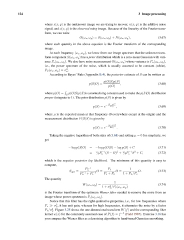
where s(x, y) is the (unknown) image we are trying to recover, n(x, y) is the additive noise
signal, and o(x, y) is the observed noisy image. Because of the linearity of the Fourier trans-
form, we can write
O(ω x ,ω y )= S(ω x ,ω y )+ N(ω x ,ω y ), (3.67)

where each quantity in the above equation is the Fourier transform of the corresponding
image.
At each frequency (ω x ,ω y ), we know from our image spectrum that the unknown trans-
form component S(ω x ,ω y ) has a prior distribution which is a zero-mean Gaussian with vari-
ance P s (ω x ,ω y ). We also have noisy measurement O(ω x ,ω y ) whose variance is P n (ω x ,ω y ),
i.e., the power spectrum of the noise, which is usually assumed to be constant (white),
2
P n (ω x ,ω y )= σ .
n
According to Bayes’ Rule (Appendix B.4), the posterior estimate of S can be written as
p(O|S)p(S)
p(S|O)= , (3.68)
p(O)

where p(O)= p(O|S)p(S) is a normalizing constant used to make the p(S|O) distribution
S
proper (integrate to 1). The prior distribution p(S) is given by
(S−μ) 2
p(S)= e − 2P s , (3.69)
where μ is the expected mean at that frequency (0 everywhere except at the origin) and the
measurement distribution P(O|S) is given by

(S−O) 2
p(S)= e − 2P n . (3.70)
Taking the negative logarithm of both sides of (3.68) and setting μ =0 for simplicity, we
get

− log p(S|O)= − log p(O|S) − log p(S)+ C (3.71)
2
2
= 1 / 2P n −1 (S − O) + / 2P s −1 S + C, (3.72)
1
which is the negative posterior log likelihood. The minimum of this quantity is easy to
compute,
P n −1 P s 1
S opt = O = O = O. (3.73)
−1 −1
P n + P s P s + P n 1+ P n /P s
The quantity
1
W(ω x ,ω y )= (3.74)
2
1+ σ /P s (ω x ,ω y )
n
is the Fourier transform of the optimum Wiener filter needed to remove the noise from an
image whose power spectrum is P s (ω x ,ω y ).
Notice that this filter has the right qualitative properties, i.e., for low frequencies where
2
P s σ , it has unit gain, whereas for high frequencies, it attenuates the noise by a factor
n
2
P s /σ . Figure 3.25 shows the one-dimensional transform W(f) and the corresponding filter
n
kernel w(x) for the commonly assumed case of P(f)= f −2 (Field 1987). Exercise 3.16 has
you compare the Wiener filter as a denoising algorithm to hand-tuned Gaussian smoothing.