Page 146 -

3.4 Fourier transforms 125

P
n
W

(a) (b)

2
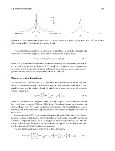
Figure 3.25 One-dimensional Wiener filter: (a) power spectrum of signal P s (f), noise level σ , and Wiener
filter transform W(f); (b) Wiener filter spatial kernel.

The methodology given above for deriving the Wiener filter can easily be extended to the
case where the observed image is a noisy blurred version of the original image,

o(x, y)= b(x, y) ∗ s(x, y)+ n(x, y), (3.75)

where b(x, y) is the known blur kernel. Rather than deriving the corresponding Wiener fil-
ter, we leave it as an exercise (Exercise 3.17), which also encourages you to compare your
de-blurring results with unsharp masking and na¨ ıve inverse filtering. More sophisticated al-
gorithms for blur removal are discussed in Sections 3.7 and 10.3.

Discrete cosine transform

The discrete cosine transform (DCT) is a variant of the Fourier transform particularly well-
suited to compressing images in a block-wise fashion. The one-dimensional DCT is com-
puted by taking the dot product of each N-wide block of pixels with a set of cosines of
different frequencies,
N−1
π 1
F(k)= cos (i + )k f(i), (3.76)
N 2
i=0
where k is the coefficient (frequency) index, and the / 2-pixel offset is used to make the
1
basis coefficients symmetric (Wallace 1991). Some of the discrete cosine basis functions are
shown in Figure 3.26. As you can see, the first basis function (the straight blue line) encodes
the average DC value in the block of pixels, while the second encodes a slightly curvy version
of the slope.
In turns out that the DCT is a good approximation to the optimal Karhunen–Lo` eve decom-
position of natural image statistics over small patches, which can be obtained by performing
a principal component analysis (PCA) of images, as described in Section 14.2.1. The KL-
transform de-correlates the signal optimally (assuming the signal is described by its spectrum)
and thus, theoretically, leads to optimal compression.
The two-dimensional version of the DCT is defined similarly,
N−1 N−1
π 1 π 1
F(k, l)= cos (i + )k cos (j + )l f(i, j). (3.77)
N 2 N 2
i=0 j=0