Page 149 -

128 3 Image processing

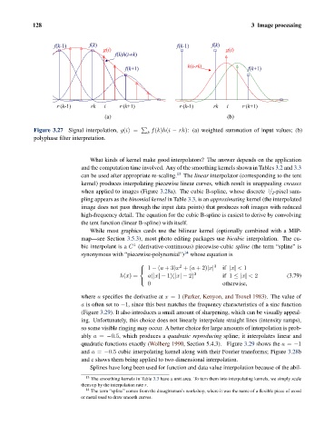
f(k-1) f(k) f(k-1) f(k)
g(i) g(i)
f(k)h(i-rk)

f(k+1) h(i-rk) f(k+1)

r·(k-1) rk i r·(k+1) r·(k-1) rk i r·(k+1)
(a) (b)

Figure 3.27 Signal interpolation, g(i)= f(k)h(i − rk): (a) weighted summation of input values; (b)
k
polyphase filter interpretation.

What kinds of kernel make good interpolators? The answer depends on the application
and the computation time involved. Any of the smoothing kernels shown in Tables 3.2 and 3.3
can be used after appropriate re-scaling. 13 The linear interpolator (corresponding to the tent
kernel) produces interpolating piecewise linear curves, which result in unappealing creases
when applied to images (Figure 3.28a). The cubic B-spline, whose discrete / 2-pixel sam-
1
pling appears as the binomial kernel in Table 3.3,is an approximating kernel (the interpolated
image does not pass through the input data points) that produces soft images with reduced
high-frequency detail. The equation for the cubic B-spline is easiest to derive by convolving
the tent function (linear B-spline) with itself.
While most graphics cards use the bilinear kernel (optionally combined with a MIP-
map—see Section 3.5.3), most photo editing packages use bicubic interpolation. The cu-
1
bic interpolant is a C (derivative-continuous) piecewise-cubic spline (the term “spline” is
14
synonymous with “piecewise-polynomial”) whose equation is
2 3
⎧
⎨ 1 − (a +3)x +(a +2)|x| if |x| < 1
h(x)= a(|x|− 1)(|x|− 2) 2 if 1 ≤|x| < 2 (3.79)
0 otherwise,
⎩
where a specifies the derivative at x =1 (Parker, Kenyon, and Troxel 1983). The value of
a is often set to −1, since this best matches the frequency characteristics of a sinc function
(Figure 3.29). It also introduces a small amount of sharpening, which can be visually appeal-
ing. Unfortunately, this choice does not linearly interpolate straight lines (intensity ramps),
so some visible ringing may occur. A better choice for large amounts of interpolation is prob-
ably a = −0.5, which produces a quadratic reproducing spline; it interpolates linear and
quadratic functions exactly (Wolberg 1990, Section 5.4.3). Figure 3.29 shows the a = −1
and a = −0.5 cubic interpolating kernel along with their Fourier transforms; Figure 3.28b
and c shows them being applied to two-dimensional interpolation.
Splines have long been used for function and data value interpolation because of the abil-
13
The smoothing kernels in Table 3.3 have a unit area. To turn them into interpolating kernels, we simply scale
them up by the interpolation rate r.
14 The term “spline” comes from the draughtsman’s workshop, where it was the name of a flexible piece of wood
or metal used to draw smooth curves.