Page 152 -

3.5 Pyramids and wavelets 131

(a) (b)

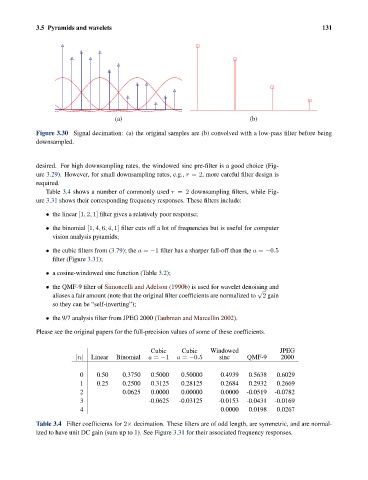
Figure 3.30 Signal decimation: (a) the original samples are (b) convolved with a low-pass filter before being
downsampled.

desired. For high downsampling rates, the windowed sinc pre-filter is a good choice (Fig-
ure 3.29). However, for small downsampling rates, e.g., r =2, more careful filter design is
required.
Table 3.4 shows a number of commonly used r =2 downsampling filters, while Fig-
ure 3.31 shows their corresponding frequency responses. These filters include:
• the linear [1, 2, 1] filter gives a relatively poor response;

• the binomial [1, 4, 6, 4, 1] filter cuts off a lot of frequencies but is useful for computer
vision analysis pyramids;
• the cubic filters from (3.79); the a = −1 filter has a sharper fall-off than the a = −0.5
filter (Figure 3.31);

• a cosine-windowed sinc function (Table 3.2);
• the QMF-9 filter of Simoncelli and Adelson (1990b) is used for wavelet denoising and
√
aliases a fair amount (note that the original filter coefficients are normalized to 2 gain
so they can be “self-inverting”);
• the 9/7 analysis filter from JPEG 2000 (Taubman and Marcellin 2002).

Please see the original papers for the full-precision values of some of these coefficients.

Cubic Cubic Windowed JPEG
|n| Linear Binomial a = −1 a = −0.5 sinc QMF-9 2000

0 0.50 0.3750 0.5000 0.50000 0.4939 0.5638 0.6029
1 0.25 0.2500 0.3125 0.28125 0.2684 0.2932 0.2669
2 0.0625 0.0000 0.00000 0.0000 -0.0519 -0.0782
3 -0.0625 -0.03125 -0.0153 -0.0431 -0.0169
4 0.0000 0.0198 0.0267
Table 3.4 Filter coefficients for 2× decimation. These filters are of odd length, are symmetric, and are normal-
ized to have unit DC gain (sum up to 1). See Figure 3.31 for their associated frequency responses.