Page 141 -

120 3 Image processing

Name Signal Transform
1.0 1.0
0.5 0.5
impulse δ(x) ⇔ 1
-1.0000 -0.5000 0.0 0.0000 0.5000 1.0000 -0.5000 0.0 0.0000 0.5000
-0.5 -0.5
1.0 1.0
shifted 0.5 −jωu 0.5
impulse -1.0000 -0.5000 0.0 0.0000 0.5000 1.0000 δ(x − u) ⇔ e -0.5000 0.0 0.0000 0.5000
-0.5 -0.5
1.0 1.0
0.5 0.5
box filter -1.0000 -0.5000 0.0 0.0000 0.5000 1.0000 box(x/a) ⇔ asinc(aω) -0.5000 0.0 0.0000 0.5000
-0.5 -0.5
1.0 1.0
0.5 2 0.5
tent -1.0000 -0.5000 0.0 0.0000 0.5000 1.0000 tent(x/a) ⇔ asinc (aω) -0.5000 0.0 0.0000 0.5000
-0.5 -0.5
1.0 1.0
0.5 √ 2π −1 0.5
Gaussian -1.0000 -0.5000 0.0 0.0000 0.5000 1.0000 G(x; σ) ⇔ σ G(ω; σ ) -0.5000 0.0 0.0000 0.5000
-0.5 -0.5
1.0 1.0
Laplacian 0.5 x 2 1 √ 2π 2 −1 0.5
( σ 4 − σ 2 )G(x; σ) − ω G(ω; σ )
of Gaussian -1.0000 -0.5000 0.0 0.0000 0.5000 1.0000 ⇔ σ -0.5000 0.0 0.0000 0.5000
-0.5 -0.5
1.0 1.0
0.5 √ 2π −1 0.5
Gabor -1.0000 -0.5000 0.0 0.0000 0.5000 1.0000 cos(ω 0 x)G(x; σ) ⇔ σ G(ω ± ω 0 ; σ ) -0.5000 0.0 0.0000 0.5000
-0.5 -0.5
1.5 1.5
1.0 (1 + γ)− 1.0
unsharp 0.5 (1 + γ)δ(x) √ 0.5
mask -1.0000 -0.5000 0.0 0.0000 0.5000 1.0000 − γG(x; σ) ⇔ 2πð G(ω; σ −1 ) -0.5000 0.0 0.0000 0.5000
σ
-0.5 -0.5
1.0 1.0
0.5 0.5
windowed rcos(x/(aW)) (see Figure 3.29)
sinc -1.0000 -0.5000 0.0 0.0000 0.5000 1.0000 sinc(x/a) ⇔ -0.5000 0.0 0.0000 0.5000
-0.5 -0.5
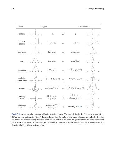
Table 3.2 Some useful (continuous) Fourier transform pairs: The dashed line in the Fourier transform of the
shifted impulse indicates its (linear) phase. All other transforms have zero phase (they are real-valued). Note that
the figures are not necessarily drawn to scale but are drawn to illustrate the general shape and characteristics of
the filter or its response. In particular, the Laplacian of Gaussian is drawn inverted because it resembles more a
“Mexican hat”, as it is sometimes called.