Page 136 -

3.3 More neighborhood operators 115

(a) (b) (c)

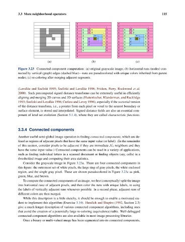
Figure 3.23 Connected component computation: (a) original grayscale image; (b) horizontal runs (nodes) con-
nected by vertical (graph) edges (dashed blue)—runs are pseudocolored with unique colors inherited from parent
nodes; (c) re-coloring after merging adjacent segments.

(Lavall´ ee and Szeliski 1995; Szeliski and Lavall´ ee 1996; Frisken, Perry, Rockwood et al.
2000). Such precomputed signed distance transforms can be extremely useful in efficiently
aligning and merging 2D curves and 3D surfaces (Huttenlocher, Klanderman, and Rucklidge
1993; Szeliski and Lavall´ ee 1996; Curless and Levoy 1996), especially if the vectorial version
of the distance transform, i.e., a pointer from each pixel or voxel to the nearest boundary or
surface element, is stored and interpolated. Signed distance fields are also an essential com-
ponent of level set evolution (Section 5.1.4), where they are called characteristic functions.

3.3.4 Connected components

Another useful semi-global image operation is finding connected components, which are de-
fined as regions of adjacent pixels that have the same input value (or label). (In the remainder
of this section, consider pixels to be adjacent if they are immediate N 4 neighbors and they
have the same input value.) Connected components can be used in a variety of applications,
such as finding individual letters in a scanned document or finding objects (say, cells) in a
thresholded image and computing their area statistics.
Consider the grayscale image in Figure 3.23a. There are four connected components in
this figure: the outermost set of white pixels, the large ring of gray pixels, the white enclosed
region, and the single gray pixel. These are shown pseudocolored in Figure 3.23c as pink,
green, blue, and brown.
To compute the connected components of an image, we first (conceptually) split the image
into horizontal runs of adjacent pixels, and then color the runs with unique labels, re-using
the labels of vertically adjacent runs whenever possible. In a second phase, adjacent runs of
different colors are then merged.
While this description is a little sketchy, it should be enough to enable a motivated stu-
dent to implement this algorithm (Exercise 3.14). Haralick and Shapiro (1992, Section 2.3)
give a much longer description of various connected component algorithms, including ones
that avoid the creation of a potentially large re-coloring (equivalence) table. Well-debugged
connected component algorithms are also available in most image processing libraries.
Once a binary or multi-valued image has been segmented into its connected components,