Page 135 -

114 3 Image processing

.
0 0 0 0 1 0 0 0 0 0 0 1 0 0 0 0 0 0 1 0 0 0 0 0 0 1 0 0
0 0 1 1 1 0 0 0 0 1 1 2 0 0 0 0 1 1 2 0 0 0 0 1 1 1 0 0
0 1 1 1 1 1 0 0 1 2 2 3 1 0 0 1 2 2 3 1 0 0 1 2 2 2 1 0
0 1 1 1 1 1 0 0 1 2 3 0 1 2 2 1 1 0 0 1 2 2 1 1 0
0 1 1 1 0 0 0 0 1 2 1 0 0 0 0 1 2 1 0 0 0
0 0 1 0 0 0 0 0 0 1 0 0 0 0 0 0 1 0 0 0 0
0 0 0 0 0 0 0 0 0 0 0 0 0 0 0 0 0 0 0 0 0
(a) (b) (c) (d)

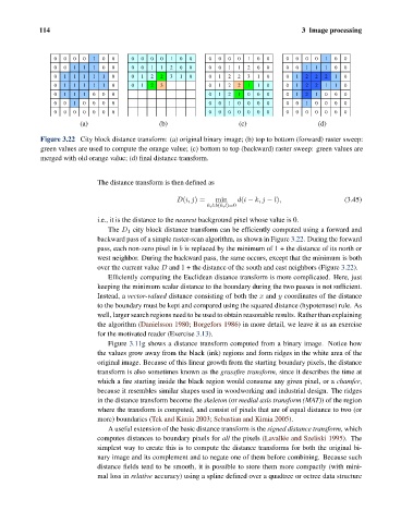
Figure 3.22 City block distance transform: (a) original binary image; (b) top to bottom (forward) raster sweep:
green values are used to compute the orange value; (c) bottom to top (backward) raster sweep: green values are
merged with old orange value; (d) final distance transform.

The distance transform is then defined as

D(i, j) = min d(i − k, j − l), (3.45)
k,l:b(k,l)=0
i.e., it is the distance to the nearest background pixel whose value is 0.
The D 1 city block distance transform can be efficiently computed using a forward and
backward pass of a simple raster-scan algorithm, as shown in Figure 3.22. During the forward
pass, each non-zero pixel in b is replaced by the minimum of 1 + the distance of its north or
west neighbor. During the backward pass, the same occurs, except that the minimum is both
over the current value D and 1 + the distance of the south and east neighbors (Figure 3.22).
Efficiently computing the Euclidean distance transform is more complicated. Here, just
keeping the minimum scalar distance to the boundary during the two passes is not sufficient.
Instead, a vector-valued distance consisting of both the x and y coordinates of the distance
to the boundary must be kept and compared using the squared distance (hypotenuse) rule. As
well, larger search regions need to be used to obtain reasonable results. Rather than explaining
the algorithm (Danielsson 1980; Borgefors 1986) in more detail, we leave it as an exercise
for the motivated reader (Exercise 3.13).
Figure 3.11g shows a distance transform computed from a binary image. Notice how
the values grow away from the black (ink) regions and form ridges in the white area of the
original image. Because of this linear growth from the starting boundary pixels, the distance
transform is also sometimes known as the grassfire transform, since it describes the time at
which a fire starting inside the black region would consume any given pixel, or a chamfer,
because it resembles similar shapes used in woodworking and industrial design. The ridges
in the distance transform become the skeleton (or medial axis transform (MAT)) of the region
where the transform is computed, and consist of pixels that are of equal distance to two (or
more) boundaries (Tek and Kimia 2003; Sebastian and Kimia 2005).
A useful extension of the basic distance transform is the signed distance transform, which
computes distances to boundary pixels for all the pixels (Lavall´ ee and Szeliski 1995). The
simplest way to create this is to compute the distance transforms for both the original bi-
nary image and its complement and to negate one of them before combining. Because such
distance fields tend to be smooth, it is possible to store them more compactly (with mini-
mal loss in relative accuracy) using a spline defined over a quadtree or octree data structure