Page 130 -

3.3 More neighborhood operators 109

. 2 1 0 1 2
1 2 1 2 4 1 2 1 2 4 2 0.1 0.3 0.4 0.3 0.1 0.0 0.0 0.0 0.0 0.2
2 1 3 5 8 2 1 3 5 8 1 0.3 0.6 0.8 0.6 0.3 0.0 0.0 0.0 0.4 0.8
1 3 7 6 9 1 3 7 6 9 0 0.4 0.8 1.0 0.8 0.4 0.0 0.0 1.0 0.8 0.4
3 4 8 6 7 3 4 8 6 7 1 0.3 0.6 0.8 0.6 0.3 0.0 0.2 0.8 0.8 1.0
4 5 7 8 9 4 5 7 8 9 2 0.1 0.3 0.4 0.3 0.1 0.2 0.4 1.0 0.8 0.4

(a) median = 4 (b) Į-mean= 4.6 (c) domain filter (d) range filter

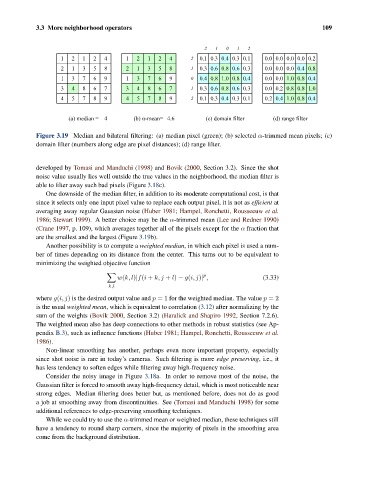
Figure 3.19 Median and bilateral filtering: (a) median pixel (green); (b) selected α-trimmed mean pixels; (c)
domain filter (numbers along edge are pixel distances); (d) range filter.

developed by Tomasi and Manduchi (1998) and Bovik (2000, Section 3.2). Since the shot
noise value usually lies well outside the true values in the neighborhood, the median filter is
able to filter away such bad pixels (Figure 3.18c).
One downside of the median filter, in addition to its moderate computational cost, is that
since it selects only one input pixel value to replace each output pixel, it is not as efficient at
averaging away regular Gaussian noise (Huber 1981; Hampel, Ronchetti, Rousseeuw et al.
1986; Stewart 1999). A better choice may be the α-trimmed mean (Lee and Redner 1990)
(Crane 1997, p. 109), which averages together all of the pixels except for the α fraction that
are the smallest and the largest (Figure 3.19b).
Another possibility is to compute a weighted median, in which each pixel is used a num-
ber of times depending on its distance from the center. This turns out to be equivalent to
minimizing the weighted objective function
p
w(k, l)|f(i + k, j + l) − g(i, j)| , (3.33)
k,l
where g(i, j) is the desired output value and p =1 for the weighted median. The value p =2
is the usual weighted mean, which is equivalent to correlation (3.12) after normalizing by the
sum of the weights (Bovik 2000, Section 3.2) (Haralick and Shapiro 1992, Section 7.2.6).
The weighted mean also has deep connections to other methods in robust statistics (see Ap-
pendix B.3), such as influence functions (Huber 1981; Hampel, Ronchetti, Rousseeuw et al.
1986).
Non-linear smoothing has another, perhaps even more important property, especially
since shot noise is rare in today’s cameras. Such filtering is more edge preserving, i.e., it
has less tendency to soften edges while filtering away high-frequency noise.
Consider the noisy image in Figure 3.18a. In order to remove most of the noise, the
Gaussian filter is forced to smooth away high-frequency detail, which is most noticeable near
strong edges. Median filtering does better but, as mentioned before, does not do as good
a job at smoothing away from discontinuities. See (Tomasi and Manduchi 1998) for some
additional references to edge-preserving smoothing techniques.
While we could try to use the α-trimmed mean or weighted median, these techniques still
have a tendency to round sharp corners, since the majority of pixels in the smoothing area
come from the background distribution.