Page 133 -

112 3 Image processing

1998; Weickert 1998). It has also been shown to be closely related to other adaptive smooth-
ing techniques (Saint-Marc, Chen, and Medioni 1991; Barash 2002; Barash and Comaniciu
2004) as well as Bayesian regularization with a non-linear smoothness term that can be de-
rived from image statistics (Scharr, Black, and Haussecker 2003).
In its general form, the range kernel r(i, j, k, l)= r( f(i, j)−f(k, l) ), which is usually
called the gain or edge-stopping function, or diffusion coefficient, can be any monotonically

increasing function with r (x) → 0 as x →∞. Black, Sapiro, Marimont et al. (1998) show
how anisotropic diffusion is equivalent to minimizing a robust penalty function on the image
gradients, which we discuss in Sections 3.7.1 and 3.7.2). Scharr, Black, and Haussecker
(2003) show how the edge-stopping function can be derived in a principled manner from
local image statistics. They also extend the diffusion neighborhood from N 4 to N 8 , which
allows them to create a diffusion operator that is both rotationally invariant and incorporates
information about the eigenvalues of the local structure tensor.
Note that, without a bias term towards the original image, anisotropic diffusion and itera-
tive adaptive smoothing converge to a constant image. Unless a small number of iterations is
used (e.g., for speed), it is usually preferable to formulate the smoothing problem as a joint
minimization of a smoothness term and a data fidelity term, as discussed in Sections 3.7.1
and 3.7.2 and by Scharr, Black, and Haussecker (2003), which introduce such a bias in a
principled manner.

3.3.2 Morphology

While non-linear filters are often used to enhance grayscale and color images, they are also
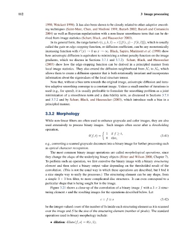
used extensively to process binary images. Such images often occur after a thresholding
operation,

1if f ≥ t,
θ(f, t)= (3.41)
0 else,
e.g., converting a scanned grayscale document into a binary image for further processing such
as optical character recognition.
The most common binary image operations are called morphological operations, since
they change the shape of the underlying binary objects (Ritter and Wilson 2000, Chapter 7).
To perform such an operation, we first convolve the binary image with a binary structuring
element and then select a binary output value depending on the thresholded result of the
convolution. (This is not the usual way in which these operations are described, but I find it
a nice simple way to unify the processes.) The structuring element can be any shape, from
a simple 3 × 3 box filter, to more complicated disc structures. It can even correspond to a
particular shape that is being sought for in the image.
Figure 3.21 shows a close-up of the convolution of a binary image f with a 3 × 3 struc-
turing element s and the resulting images for the operations described below. Let
c = f ⊗ s (3.42)

be the integer-valued count of the number of 1s inside each structuring element as it is scanned
over the image and S be the size of the structuring element (number of pixels). The standard
operations used in binary morphology include:

• dilation: dilate(f, s)= θ(c, 1);