Page 128 -

3.2 Linear filtering 107

3 2 7 2 3 3 5 12 14 17 3 5 12 14 17
1 5 1 3 4 4 11 19 2431 4 11192431
5 1 3 5 1 9 17 28 38 46 9 17 28 38 46

4 3 2 1 6 13 24 37 48 62 13 24 37 48 62
2 4 1 4 8 15 30 44 59 81 15 30 44 59 81

(a) S = 24 (b) s = 28 (c) S = 24

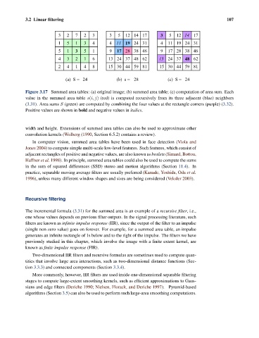
Figure 3.17 Summed area tables: (a) original image; (b) summed area table; (c) computation of area sum. Each
value in the summed area table s(i, j) (red) is computed recursively from its three adjacent (blue) neighbors
(3.31). Area sums S (green) are computed by combining the four values at the rectangle corners (purple) (3.32).
Positive values are shown in bold and negative values in italics.

width and height. Extensions of summed area tables can also be used to approximate other
convolution kernels (Wolberg (1990, Section 6.5.2) contains a review).
In computer vision, summed area tables have been used in face detection (Viola and
Jones 2004) to compute simple multi-scale low-level features. Such features, which consist of
adjacent rectangles of positive and negative values, are also known as boxlets (Simard, Bottou,
Haffner et al. 1998). In principle, summed area tables could also be used to compute the sums
in the sum of squared differences (SSD) stereo and motion algorithms (Section 11.4). In
practice, separable moving average filters are usually preferred (Kanade, Yoshida, Oda et al.
1996), unless many different window shapes and sizes are being considered (Veksler 2003).

Recursive filtering

The incremental formula (3.31) for the summed area is an example of a recursive filter, i.e.,
one whose values depends on previous filter outputs. In the signal processing literature, such
filters are known as infinite impulse response (IIR), since the output of the filter to an impulse
(single non-zero value) goes on forever. For example, for a summed area table, an impulse
generates an infinite rectangle of 1s below and to the right of the impulse. The filters we have
previously studied in this chapter, which involve the image with a finite extent kernel, are
known as finite impulse response (FIR).
Two-dimensional IIR filters and recursive formulas are sometimes used to compute quan-
tities that involve large area interactions, such as two-dimensional distance functions (Sec-
tion 3.3.3) and connected components (Section 3.3.4).
More commonly, however, IIR filters are used inside one-dimensional separable filtering
stages to compute large-extent smoothing kernels, such as efficient approximations to Gaus-
sians and edge filters (Deriche 1990; Nielsen, Florack, and Deriche 1997). Pyramid-based
algorithms (Section 3.5) can also be used to perform such large-area smoothing computations.