Page 131 -

110 3 Image processing

Bilateral filtering

What if we were to combine the idea of a weighted filter kernel with a better version of outlier
rejection? What if instead of rejecting a fixed percentage α, we simply reject (in a soft way)
pixels whose values differ too much from the central pixel value? This is the essential idea in
bilateral filtering, which was first popularized in the computer vision community by Tomasi
and Manduchi (1998). Chen, Paris, and Durand (2007) and Paris, Kornprobst, Tumblin et al.
(2008) cite similar earlier work (Aurich and Weule 1995; Smith and Brady 1997) as well as
the wealth of subsequent applications in computer vision and computational photography.
In the bilateral filter, the output pixel value depends on a weighted combination of neigh-
boring pixel values
f(k, l)w(i, j, k, l)

k,l
g(i, j)= . (3.34)
w(i, j, k, l)
k,l
The weighting coefficient w(i, j, k, l) depends on the product of a domain kernel (Figure 3.19c),
2 2
(i − k) +(j − l)
d(i, j, k, l) = exp − 2 , (3.35)
2σ
d
and a data-dependent range kernel (Figure 3.19d),
2

f(i, j) − f(k, l)
r(i, j, k, l) = exp − 2 . (3.36)
2σ r
When multiplied together, these yield the data-dependent bilateral weight function
2 2 2
(i − k) +(j − l) f(i, j) − f(k, l)
w(i, j, k, l) = exp − 2 − 2 . (3.37)
2σ 2σ
d r
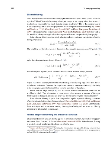
Figure 3.20 shows an example of the bilateral filtering of a noisy step edge. Note how the do-
main kernel is the usual Gaussian, the range kernel measures appearance (intensity) similarity
to the center pixel, and the bilateral filter kernel is a product of these two.
Notice that the range filter (3.36) uses the vector distance between the center and the
neighboring pixel. This is important in color images, since an edge in any one of the color
bands signals a change in material and hence the need to downweight a pixel’s influence. 5
Since bilateral filtering is quite slow compared to regular separable filtering, a number
of acceleration techniques have been developed (Durand and Dorsey 2002; Paris and Durand
2006; Chen, Paris, and Durand 2007; Paris, Kornprobst, Tumblin et al. 2008). Unfortunately,
these techniques tend to use more memory than regular filtering and are hence not directly
applicable to filtering full-color images.

Iterated adaptive smoothing and anisotropic diffusion
Bilateral (and other) filters can also be applied in an iterative fashion, especially if an appear-
ance more like a “cartoon” is desired (Tomasi and Manduchi 1998). When iterated filtering
is applied, a much smaller neighborhood can often be used.
5
Tomasi and Manduchi (1998) show that using the vector distance (as opposed to filtering each color band
separately) reduces color fringing effects. They also recommend taking the color difference in the more perceptually
uniform CIELAB color space (see Section 2.3.2).