Page 134 -

3.3 More neighborhood operators 113

(a) (b) (c) (d) (e) (f)
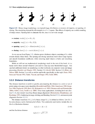
Figure 3.21 Binary image morphology: (a) original image; (b) dilation; (c) erosion; (d) majority; (e) opening; (f)
closing. The structuring element for all examples is a 5 × 5 square. The effects of majority are a subtle rounding
of sharp corners. Opening fails to eliminate the dot, since it is not wide enough.

• erosion: erode(f, s)= θ(c, S);

• majority: maj(f, s)= θ(c, S/2);

• opening: open(f, s) = dilate(erode(f, s),s);

• closing: close(f, s) = erode(dilate(f, s),s).

As we can see from Figure 3.21, dilation grows (thickens) objects consisting of 1s, while
erosion shrinks (thins) them. The opening and closing operations tend to leave large regions
and smooth boundaries unaffected, while removing small objects or holes and smoothing
boundaries.
While we will not use mathematical morphology much in the rest of this book, it is a
handy tool to have around whenever you need to clean up some thresholded images. You
can find additional details on morphology in other textbooks on computer vision and image
processing (Haralick and Shapiro 1992, Section 5.2) (Bovik 2000, Section 2.2) (Ritter and
Wilson 2000, Section 7) as well as articles and books specifically on this topic (Serra 1982;
Serra and Vincent 1992; Yuille, Vincent, and Geiger 1992; Soille 2006).

3.3.3 Distance transforms

The distance transform is useful in quickly precomputing the distance to a curve or set of
points using a two-pass raster algorithm (Rosenfeld and Pfaltz 1966; Danielsson 1980; Borge-
fors 1986; Paglieroni 1992; Breu, Gil, Kirkpatrick et al. 1995; Felzenszwalb and Huttenlocher
2004a; Fabbri, Costa, Torelli et al. 2008). It has many applications, including level sets (Sec-
tion 5.1.4), fast chamfer matching (binary image alignment) (Huttenlocher, Klanderman, and
Rucklidge 1993), feathering in image stitching and blending (Section 9.3.2), and nearest point
alignment (Section 12.2.1).
The distance transform D(i, j) of a binary image b(i, j) is defined as follows. Let d(k, l)
be some distance metric between pixel offsets. Two commonly used metrics include the city
block or Manhattan distance
d 1 (k, l)= |k| + |l| (3.43)

and the Euclidean distance

2
2
d 2 (k, l)= k + l . (3.44)