Page 139 -

118 3 Image processing

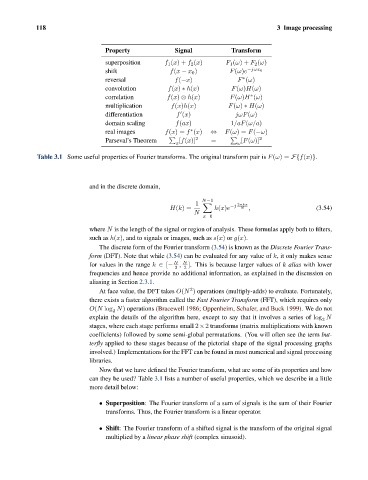
Property Signal Transform
superposition f 1 (x)+ f 2 (x) F 1 (ω)+ F 2 (ω)
shift f(x − x 0 ) F(ω)e −jωx 0
reversal f(−x) F (ω)
∗
convolution f(x) ∗ h(x) F(ω)H(ω)
correlation f(x) ⊗ h(x) F(ω)H (ω)
∗
multiplication f(x)h(x) F(ω) ∗ H(ω)
differentiation f (x) jωF(ω)

domain scaling f(ax) 1/aF(ω/a)
∗
real images f(x)= f (x) ⇔ F(ω)= F(−ω)
Parseval’s Theorem [f(x)] 2 = [F(ω)] 2
x ω
Table 3.1 Some useful properties of Fourier transforms. The original transform pair is F(ω)= F{f(x)}.

and in the discrete domain,

N−1
1 2πkx
H(k)= h(x)e −j N , (3.54)
N
x=0
where N is the length of the signal or region of analysis. These formulas apply both to filters,
such as h(x), and to signals or images, such as s(x) or g(x).
The discrete form of the Fourier transform (3.54) is known as the Discrete Fourier Trans-
form (DFT). Note that while (3.54) can be evaluated for any value of k, it only makes sense
N
for values in the range k ∈ [− , N ]. This is because larger values of k alias with lower
2 2
frequencies and hence provide no additional information, as explained in the discussion on
aliasing in Section 2.3.1.
2
At face value, the DFT takes O(N ) operations (multiply-adds) to evaluate. Fortunately,
there exists a faster algorithm called the Fast Fourier Transform (FFT), which requires only
O(N log N) operations (Bracewell 1986; Oppenheim, Schafer, and Buck 1999). We do not
2
explain the details of the algorithm here, except to say that it involves a series of log N
2
stages, where each stage performs small 2×2 transforms (matrix multiplications with known
coefficients) followed by some semi-global permutations. (You will often see the term but-
terfly applied to these stages because of the pictorial shape of the signal processing graphs
involved.) Implementations for the FFT can be found in most numerical and signal processing
libraries.
Now that we have defined the Fourier transform, what are some of its properties and how
can they be used? Table 3.1 lists a number of useful properties, which we describe in a little
more detail below:

• Superposition: The Fourier transform of a sum of signals is the sum of their Fourier
transforms. Thus, the Fourier transform is a linear operator.

• Shift: The Fourier transform of a shifted signal is the transform of the original signal
multiplied by a linear phase shift (complex sinusoid).