Page 158 -

3.5 Pyramids and wavelets 137

LH 0 HH 0 LH 0 HH 0
H Ļ2 Q 2 F
HL 0 HL 0

L Ļ2 L 1 L 1 2 I

(a)

H v Ļ2 v HH 0 Q HH 0 2 v F v
H h Ļ2 h 2 h F h
Q
L v Ļ2 v HL 0 HL 0 2 v I v
H v Ļ2 v LH 0 Q LH 0 2 v F v
L h Ļ2 h 2 h I h
L v Ļ2 v L 1 L 1 2 v I v

(b)

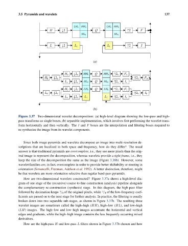
Figure 3.37 Two-dimensional wavelet decomposition: (a) high-level diagram showing the low-pass and high-
pass transforms as single boxes; (b) separable implementation, which involves first performing the wavelet trans-
form horizontally and then vertically. The I and F boxes are the interpolation and filtering boxes required to
re-synthesize the image from its wavelet components.

Since both image pyramids and wavelets decompose an image into multi-resolution de-
scriptions that are localized in both space and frequency, how do they differ? The usual
answer is that traditional pyramids are overcomplete, i.e., they use more pixels than the orig-
inal image to represent the decomposition, whereas wavelets provide a tight frame, i.e., they
keep the size of the decomposition the same as the image (Figure 3.36b). However, some
wavelet families are, in fact, overcomplete in order to provide better shiftability or steering in
orientation (Simoncelli, Freeman, Adelson et al. 1992). A better distinction, therefore, might
be that wavelets are more orientation selective than regular band-pass pyramids.
How are two-dimensional wavelets constructed? Figure 3.37a shows a high-level dia-
gram of one stage of the (recursive) coarse-to-fine construction (analysis) pipeline alongside
the complementary re-construction (synthesis) stage. In this diagram, the high-pass filter
followed by decimation keeps / 4 of the original pixels, while / 4 of the low-frequency coef-
1
3
ficients are passed on to the next stage for further analysis. In practice, the filtering is usually
broken down into two separable sub-stages, as shown in Figure 3.37b. The resulting three
wavelet images are sometimes called the high–high (HH), high–low (HL), and low–high
(LH) images. The high–low and low–high images accentuate the horizontal and vertical
edges and gradients, while the high–high image contains the less frequently occurring mixed
derivatives.
How are the high-pass H and low-pass L filters shown in Figure 3.37b chosen and how