Page 189 -

168 3 Image processing

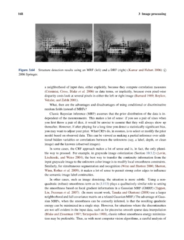
Figure 3.64 Structure detection results using an MRF (left) and a DRF (right) (Kumar and Hebert 2006) c
2006 Springer.

a neighborhood of input data, either explicitly, because they compute correlation measures
(Criminisi, Cross, Blake et al. 2006) as data terms, or implicitly, because even pixel-wise
disparity costs look at several pixels in either the left or right image (Barnard 1989; Boykov,
Veksler, and Zabih 2001).
What, then are the advantages and disadvantages of using conditional or discriminative
random fields instead of MRFs?
Classic Bayesian inference (MRF) assumes that the prior distribution of the data is in-
dependent of the measurements. This makes a lot of sense: if you see a pair of sixes when
you first throw a pair of dice, it would be unwise to assume that they will always show up
thereafter. However, if after playing for a long time you detect a statistically significant bias,
you may want to adjust your prior. What CRFs do, in essence, is to select or modify the prior
model based on observed data. This can be viewed as making a partial inference over addi-
tional hidden variables or correlations between the unknowns (say, a label, depth, or clean
image) and the knowns (observed images).
In some cases, the CRF approach makes a lot of sense and is, in fact, the only plausi-
ble way to proceed. For example, in grayscale image colorization (Section 10.3.2)(Levin,
Lischinski, and Weiss 2004), the best way to transfer the continuity information from the
input grayscale image to the unknown color image is to modify local smoothness constraints.
Similarly, for simultaneous segmentation and recognition (Winn and Shotton 2006; Shotton,
Winn, Rother et al. 2009), it makes a lot of sense to permit strong color edges to influence
the semantic image label continuities.
In other cases, such as image denoising, the situation is more subtle. Using a non-
quadratic (robust) smoothness term as in (3.113) plays a qualitatively similar role to setting
the smoothness based on local gradient information in a Gaussian MRF (GMRF) (Tappen,
Liu, Freeman et al. 2007). (In more recent work, Tanaka and Okutomi (2008) use a larger
neighborhood and full covariance matrix on a related Gaussian MRF.) The advantage of Gaus-
sian MRFs, when the smoothness can be correctly inferred, is that the resulting quadratic
energy can be minimized in a single step. However, for situations where the discontinuities
are not self-evident in the input data, such as for piecewise-smooth sparse data interpolation
(Blake and Zisserman 1987; Terzopoulos 1988), classic robust smoothness energy minimiza-
tion may be preferable. Thus, as with most computer vision algorithms, a careful analysis of