Page 187 -

166 3 Image processing

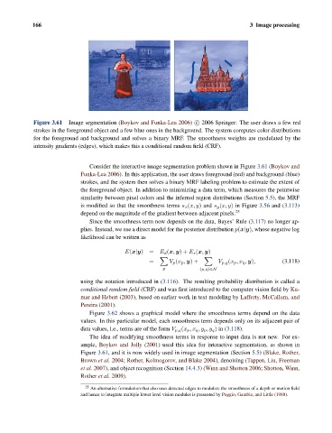
Figure 3.61 Image segmentation (Boykov and Funka-Lea 2006) c 2006 Springer: The user draws a few red
strokes in the foreground object and a few blue ones in the background. The system computes color distributions
for the foreground and background and solves a binary MRF. The smoothness weights are modulated by the
intensity gradients (edges), which makes this a conditional random field (CRF).

Consider the interactive image segmentation problem shown in Figure 3.61 (Boykov and
Funka-Lea 2006). In this application, the user draws foreground (red) and background (blue)
strokes, and the system then solves a binary MRF labeling problem to estimate the extent of
the foreground object. In addition to minimizing a data term, which measures the pointwise
similarity between pixel colors and the inferred region distributions (Section 5.5), the MRF
is modified so that the smoothness terms s x (x, y) and s y (x, y) in Figure 3.56 and (3.113)
depend on the magnitude of the gradient between adjacent pixels. 25
Since the smoothness term now depends on the data, Bayes’ Rule (3.117) no longer ap-
plies. Instead, we use a direct model for the posterior distribution p(x|y), whose negative log
likelihood can be written as

E(x|y)= E d (x, y)+ E s (x, y)

= V p (x p , y)+ V p,q (x p ,x q , y), (3.118)
p (p,q)∈N

using the notation introduced in (3.116). The resulting probability distribution is called a
conditional random field (CRF) and was first introduced to the computer vision field by Ku-
mar and Hebert (2003), based on earlier work in text modeling by Lafferty, McCallum, and
Pereira (2001).
Figure 3.62 shows a graphical model where the smoothness terms depend on the data
values. In this particular model, each smoothness term depends only on its adjacent pair of
data values, i.e., terms are of the form V p,q (x p ,x q ,y p ,y q ) in (3.118).
The idea of modifying smoothness terms in response to input data is not new. For ex-
ample, Boykov and Jolly (2001) used this idea for interactive segmentation, as shown in
Figure 3.61, and it is now widely used in image segmentation (Section 5.5)(Blake, Rother,
Brown et al. 2004; Rother, Kolmogorov, and Blake 2004), denoising (Tappen, Liu, Freeman
et al. 2007), and object recognition (Section 14.4.3)(Winn and Shotton 2006; Shotton, Winn,
Rother et al. 2009).

25 An alternative formulation that also uses detected edges to modulate the smoothness of a depth or motion field
and hence to integrate multiple lower level vision modules is presented by Poggio, Gamble, and Little (1988).