Page 186 -

3.7 Global optimization 165

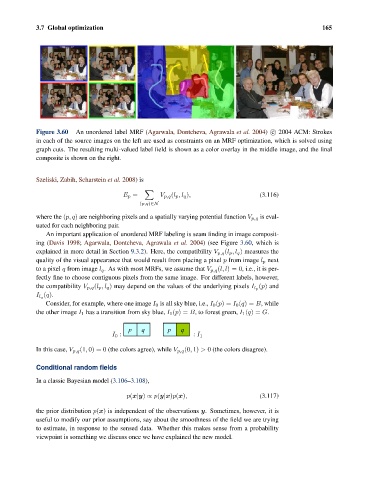
Figure 3.60 An unordered label MRF (Agarwala, Dontcheva, Agrawala et al. 2004) c 2004 ACM: Strokes
in each of the source images on the left are used as constraints on an MRF optimization, which is solved using
graph cuts. The resulting multi-valued label field is shown as a color overlay in the middle image, and the final
composite is shown on the right.

Szeliski, Zabih, Scharstein et al. 2008)is

E p = V p,q (l p ,l q ), (3.116)
(p,q)∈N
where the (p, q) are neighboring pixels and a spatially varying potential function V p,q is eval-
uated for each neighboring pair.
An important application of unordered MRF labeling is seam finding in image composit-
ing (Davis 1998; Agarwala, Dontcheva, Agrawala et al. 2004) (see Figure 3.60, which is
explained in more detail in Section 9.3.2). Here, the compatibility V p,q (l p ,l q ) measures the
quality of the visual appearance that would result from placing a pixel p from image l p next
to a pixel q from image l q . As with most MRFs, we assume that V p,q (l, l)=0, i.e., it is per-
fectly fine to choose contiguous pixels from the same image. For different labels, however,
(p) and
the compatibility V p,q (l p ,l q ) may depend on the values of the underlying pixels I l p
(q).
I l q
Consider, for example, where one image I 0 is all sky blue, i.e., I 0 (p)= I 0 (q)= B, while
the other image I 1 has a transition from sky blue, I 1 (p)= B, to forest green, I 1 (q)= G.

p q p q
I 0 : : I 1

In this case, V p,q (1, 0) = 0 (the colors agree), while V p,q (0, 1) > 0 (the colors disagree).

Conditional random fields
In a classic Bayesian model (3.106–3.108),

p(x|y) ∝ p(y|x)p(x), (3.117)

the prior distribution p(x) is independent of the observations y. Sometimes, however, it is
useful to modify our prior assumptions, say about the smoothness of the field we are trying
to estimate, in response to the sensed data. Whether this makes sense from a probability
viewpoint is something we discuss once we have explained the new model.