Page 188 -

3.7 Global optimization 167

f (i, j+1)

d (i, j) f (i+1, j+1)

w(i, j) s y(i, j)

f (i, j) s x(i, j) f (i+1, j)

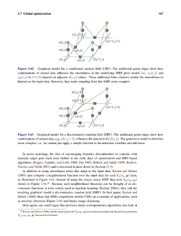
Figure 3.62 Graphical model for a conditional random field (CRF). The additional green edges show how
combinations of sensed data influence the smoothness in the underlying MRF prior model, i.e., s x (i, j) and
s y (i, j) in (3.113) depend on adjacent d(i, j) values. These additional links (factors) enable the smoothness to
depend on the input data. However, they make sampling from this MRF more complex.

d (i, j+1)

f (i, j+1)

d (i, j) f (i+1, j+1)

w(i, j) s y(i, j)

f (i, j) s x(i, j) f (i+1, j)

Figure 3.63 Graphical model for a discriminative random field (DRF). The additional green edges show how
combinations of sensed data, e.g., d(i, j+1), influence the data term for f(i, j). The generative model is therefore
more complex, i.e., we cannot just apply a simple function to the unknown variables and add noise.

In stereo matching, the idea of encouraging disparity discontinuities to coincide with
intensity edges goes back even further to the early days of optimization and MRF-based
algorithms (Poggio, Gamble, and Little 1988; Fua 1993; Bobick and Intille 1999; Boykov,
Veksler, and Zabih 2001) and is discussed in more detail in (Section 11.5).
In addition to using smoothness terms that adapt to the input data, Kumar and Hebert
(2003) also compute a neighborhood function over the input data for each V p (x p , y) term,
as illustrated in Figure 3.63, instead of using the classic unary MRF data term V p (x p ,y p )
shown in Figure 3.56. 26 Because such neighborhood functions can be thought of as dis-
criminant functions (a term widely used in machine learning (Bishop 2006)), they call the
resulting graphical model a discriminative random field (DRF). In their paper, Kumar and
Hebert (2006) show that DRFs outperform similar CRFs on a number of applications, such
as structure detection (Figure 3.64) and binary image denoising.
Here again, one could argue that previous stereo correspondence algorithms also look at

26 Kumar and Hebert (2006) call the unary potentials V p(x p, y) association potentials and the pairwise potentials
V p,q (x p,y q , y) interaction potentials.