Page 185 -

164 3 Image processing

d (i, j+1)

f (i, j+1)

d (i, j) f (i+1, j+1)

w(i, j) s y(i, j)

f (i, j) s x(i, j) f (i+1, j)

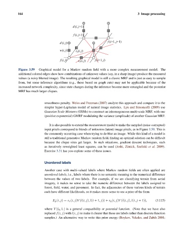
Figure 3.59 Graphical model for a Markov random field with a more complex measurement model. The
additional colored edges show how combinations of unknown values (say, in a sharp image) produce the measured
values (a noisy blurred image). The resulting graphical model is still a classic MRF and is just as easy to sample
from, but some inference algorithms (e.g., those based on graph cuts) may not be applicable because of the
increased network complexity, since state changes during the inference become more entangled and the posterior
MRF has much larger cliques.

smoothness penalty. Weiss and Freeman (2007) analyze this approach and compare it to the
simpler hyper-Laplacian model of natural image statistics. Lyu and Simoncelli (2009) use
Gaussian Scale Mixtures (GSMs) to construct an inhomogeneous multi-scale MRF, with one
(positive exponential) GMRF modulating the variance (amplitude) of another Gaussian MRF.

It is also possible to extend the measurement model to make the sampled (noise-corrupted)
input pixels correspond to blends of unknown (latent) image pixels, as in Figure 3.59. This is
the commonly occurring case when trying to de-blur an image. While this kind of a model is
still a traditional generative Markov random field, finding an optimal solution can be difficult
because the clique sizes get larger. In such situations, gradient descent techniques, such
as iteratively reweighted least squares, can be used (Joshi, Zitnick, Szeliski et al. 2009).
Exercise 3.31 has you explore some of these issues.

Unordered labels

Another case with multi-valued labels where Markov random fields are often applied are
unordered labels, i.e., labels where there is no semantic meaning to the numerical difference
between the values of two labels. For example, if we are classifying terrain from aerial
imagery, it makes no sense to take the numeric difference between the labels assigned to
forest, field, water, and pavement. In fact, the adjacencies of these various kinds of terrain
each have different likelihoods, so it makes more sense to use a prior of the form

E p (i, j)= s x (i, j)V (l(i, j),l(i +1,j)) + s y (i, j)V (l(i, j),l(i, j + 1)), (3.115)

where V (l 0 ,l 1 ) is a general compatibility or potential function. (Note that we have also
replaced f(i, j) with l(i, j) to make it clearer that these are labels rather than discrete function
samples.) An alternative way to write this prior energy (Boykov, Veksler, and Zabih 2001;