Page 183 -

162 3 Image processing

(a) (b) (c) (d)

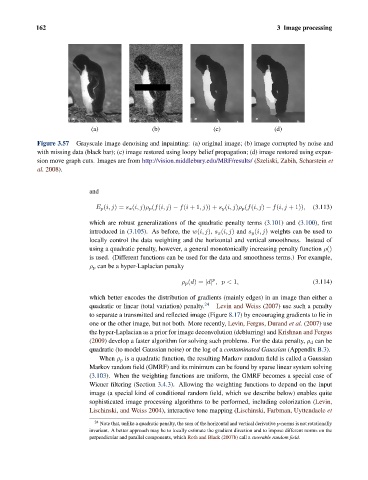
Figure 3.57 Grayscale image denoising and inpainting: (a) original image; (b) image corrupted by noise and
with missing data (black bar); (c) image restored using loopy belief propagation; (d) image restored using expan-
sion move graph cuts. Images are from http://vision.middlebury.edu/MRF/results/ (Szeliski, Zabih, Scharstein et
al. 2008).

and

E p (i, j)= s x (i, j)ρ p (f(i, j) − f(i +1,j)) + s y (i, j)ρ p (f(i, j) − f(i, j + 1)), (3.113)

which are robust generalizations of the quadratic penalty terms (3.101) and (3.100), first
introduced in (3.105). As before, the w(i, j), s x (i, j) and s y (i, j) weights can be used to
locally control the data weighting and the horizontal and vertical smoothness. Instead of
using a quadratic penalty, however, a general monotonically increasing penalty function ρ()
is used. (Different functions can be used for the data and smoothness terms.) For example,
ρ p can be a hyper-Laplacian penalty

p
ρ p (d)= |d| ,p < 1, (3.114)
which better encodes the distribution of gradients (mainly edges) in an image than either a
quadratic or linear (total variation) penalty. 24 Levin and Weiss (2007) use such a penalty
to separate a transmitted and reflected image (Figure 8.17) by encouraging gradients to lie in
one or the other image, but not both. More recently, Levin, Fergus, Durand et al. (2007) use
the hyper-Laplacian as a prior for image deconvolution (deblurring) and Krishnan and Fergus
(2009) develop a faster algorithm for solving such problems. For the data penalty, ρ d can be
quadratic (to model Gaussian noise) or the log of a contaminated Gaussian (Appendix B.3).
When ρ p is a quadratic function, the resulting Markov random field is called a Gaussian
Markov random field (GMRF) and its minimum can be found by sparse linear system solving
(3.103). When the weighting functions are uniform, the GMRF becomes a special case of
Wiener filtering (Section 3.4.3). Allowing the weighting functions to depend on the input
image (a special kind of conditional random field, which we describe below) enables quite
sophisticated image processing algorithms to be performed, including colorization (Levin,
Lischinski, and Weiss 2004), interactive tone mapping (Lischinski, Farbman, Uyttendaele et
24
Note that, unlike a quadratic penalty, the sum of the horizontal and vertical derivative p-norms is not rotationally
invariant. A better approach may be to locally estimate the gradient direction and to impose different norms on the
perpendicular and parallel components, which Roth and Black (2007b) call a steerable random field.