Page 178 -

3.7 Global optimization 157

f (i, j+1)

d (i, j) f (i+1, j+1)

w(i, j) s y(i, j)

f (i, j) s x(i, j) f (i+1, j)

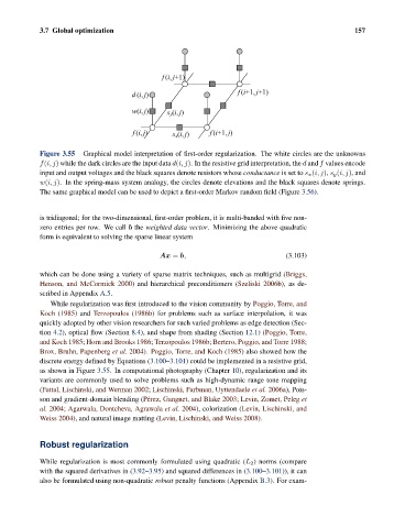
Figure 3.55 Graphical model interpretation of first-order regularization. The white circles are the unknowns
f(i, j) while the dark circles are the input data d(i, j). In the resistive grid interpretation, the d and f values encode
input and output voltages and the black squares denote resistors whose conductance is set to s x (i, j), s y (i, j), and
w(i, j). In the spring-mass system analogy, the circles denote elevations and the black squares denote springs.
The same graphical model can be used to depict a first-order Markov random field (Figure 3.56).

is tridiagonal; for the two-dimensional, first-order problem, it is multi-banded with five non-
zero entries per row. We call b the weighted data vector. Minimizing the above quadratic
form is equivalent to solving the sparse linear system

Ax = b, (3.103)

which can be done using a variety of sparse matrix techniques, such as multigrid (Briggs,
Henson, and McCormick 2000) and hierarchical preconditioners (Szeliski 2006b), as de-
scribed in Appendix A.5.
While regularization was first introduced to the vision community by Poggio, Torre, and
Koch (1985) and Terzopoulos (1986b) for problems such as surface interpolation, it was
quickly adopted by other vision researchers for such varied problems as edge detection (Sec-
tion 4.2), optical flow (Section 8.4), and shape from shading (Section 12.1)(Poggio, Torre,
and Koch 1985; Horn and Brooks 1986; Terzopoulos 1986b; Bertero, Poggio, and Torre 1988;
Brox, Bruhn, Papenberg et al. 2004). Poggio, Torre, and Koch (1985) also showed how the
discrete energy defined by Equations (3.100–3.101) could be implemented in a resistive grid,
as shown in Figure 3.55. In computational photography (Chapter 10), regularization and its
variants are commonly used to solve problems such as high-dynamic range tone mapping
(Fattal, Lischinski, and Werman 2002; Lischinski, Farbman, Uyttendaele et al. 2006a), Pois-
son and gradient-domain blending (P´ erez, Gangnet, and Blake 2003; Levin, Zomet, Peleg et
al. 2004; Agarwala, Dontcheva, Agrawala et al. 2004), colorization (Levin, Lischinski, and
Weiss 2004), and natural image matting (Levin, Lischinski, and Weiss 2008).

Robust regularization

While regularization is most commonly formulated using quadratic (L 2 ) norms (compare
with the squared derivatives in (3.92–3.95) and squared differences in (3.100–3.101)), it can
also be formulated using non-quadratic robust penalty functions (Appendix B.3). For exam-