Page 174 -

3.7 Global optimization 153

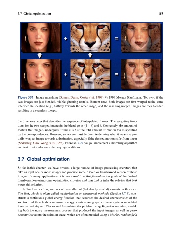
Figure 3.53 Image morphing (Gomes, Darsa, Costa et al. 1999) c 1999 Morgan Kaufmann. Top row: if the
two images are just blended, visible ghosting results. Bottom row: both images are first warped to the same
intermediate location (e.g., halfway towards the other image) and the resulting warped images are then blended
resulting in a seamless morph.

the time parameter that describes the sequence of interpolated frames. The weighting func-
tions for the two warped images in the blend go as (1 − t) and t. Conversely, the amount of
motion that image 0 undergoes at time t is t of the total amount of motion that is specified
by the correspondences. However, some care must be taken in defining what it means to par-
tially warp an image towards a destination, especially if the desired motion is far from linear
(Sederberg, Gao, Wang et al. 1993). Exercise 3.25 has you implement a morphing algorithm
and test it out under such challenging conditions.

3.7 Global optimization

So far in this chapter, we have covered a large number of image processing operators that
take as input one or more images and produce some filtered or transformed version of these
images. In many applications, it is more useful to first formulate the goals of the desired
transformation using some optimization criterion and then find or infer the solution that best
meets this criterion.
In this final section, we present two different (but closely related) variants on this idea.
The first, which is often called regularization or variational methods (Section 3.7.1), con-
structs a continuous global energy function that describes the desired characteristics of the
solution and then finds a minimum energy solution using sparse linear systems or related
iterative techniques. The second formulates the problem using Bayesian statistics, model-
ing both the noisy measurement process that produced the input images as well as prior
assumptions about the solution space, which are often encoded using a Markov random field