Page 175 -

154 3 Image processing

(a) (b)

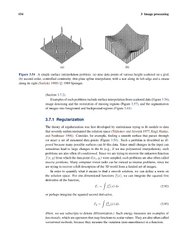
Figure 3.54 A simple surface interpolation problem: (a) nine data points of various height scattered on a grid;
(b) second-order, controlled-continuity, thin-plate spline interpolator, with a tear along its left edge and a crease
along its right (Szeliski 1989) c 1989 Springer.

(Section 3.7.2).
Examples of such problems include surface interpolation from scattered data (Figure 3.54),
image denoising and the restoration of missing regions (Figure 3.57), and the segmentation
of images into foreground and background regions (Figure 3.61).

3.7.1 Regularization

The theory of regularization was first developed by statisticians trying to fit models to data
that severely underconstrained the solution space (Tikhonov and Arsenin 1977; Engl, Hanke,
and Neubauer 1996). Consider, for example, finding a smooth surface that passes through
(or near) a set of measured data points (Figure 3.54). Such a problem is described as ill-
posed because many possible surfaces can fit this data. Since small changes in the input can
sometimes lead to large changes in the fit (e.g., if we use polynomial interpolation), such
problems are also often ill-conditioned. Since we are trying to recover the unknown function
f(x, y) from which the data point d(x i ,y i ) were sampled, such problems are also often called
inverse problems. Many computer vision tasks can be viewed as inverse problems, since we
are trying to recover a full description of the 3D world from a limited set of images.
In order to quantify what it means to find a smooth solution, we can define a norm on
the solution space. For one-dimensional functions f(x), we can integrate the squared first
derivative of the function,

2
E 1 = f (x) dx (3.92)
x
or perhaps integrate the squared second derivative,

2
E 2 = f (x) dx. (3.93)
xx
(Here, we use subscripts to denote differentiation.) Such energy measures are examples of
functionals, which are operators that map functions to scalar values. They are also often called
variational methods, because they measure the variation (non-smoothness) in a function.