Page 176 -

3.7 Global optimization 155

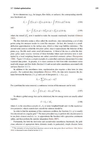
In two dimensions (e.g., for images, flow fields, or surfaces), the corresponding smooth-
ness functionals are

2
2
2
E 1 = f (x, y)+ f (x, y) dx dy = ∇f(x, y) dx dy (3.94)
x
y
and

2
2
2
E 2 = f (x, y)+2f (x, y)+ f (x, y) dx dy, (3.95)
xx xy yy
where the mixed 2f 2 term is needed to make the measure rotationally invariant (Grimson
xy
1983).
The first derivative norm is often called the membrane, since interpolating a set of data
points using this measure results in a tent-like structure. (In fact, this formula is a small-
deflection approximation to the surface area, which is what soap bubbles minimize.) The
second-order norm is called the thin-plate spline, since it approximates the behavior of thin
plates (e.g., flexible steel) under small deformations. A blend of the two is called the thin-
plate spline under tension; versions of these formulas where each derivative term is mul-
tiplied by a local weighting function are called controlled-continuity splines (Terzopoulos
1988). Figure 3.54 shows a simple example of a controlled-continuity interpolator fit to nine
scattered data points. In practice, it is more common to find first-order smoothness terms
used with images and flow fields (Section 8.4) and second-order smoothness associated with
surfaces (Section 12.3.1).
In addition to the smoothness term, regularization also requires a data term (or data
penalty). For scattered data interpolation (Nielson 1993), the data term measures the dis-
tance between the function f(x, y) and a set of data points d i = d(x i ,y i ),

2
E d = [f(x i ,y i ) − d i ] . (3.96)
i
For a problem like noise removal, a continuous version of this measure can be used,

2
E d = [f(x, y) − d(x, y)] dx dy. (3.97)
To obtain a global energy that can be minimized, the two energy terms are usually added
together,
E = E d + λE s , (3.98)
where E s is the smoothness penalty (E 1 , E 2 or some weighted blend) and λ is the regulariza-
tion parameter, which controls how smooth the solution should be.
In order to find the minimum of this continuous problem, the function f(x, y) is usually
first discretized on a regular grid. 21 The most principled way to perform this discretization is
to use finite element analysis, i.e., to approximate the function with a piecewise continuous
spline, and then perform the analytic integration (Bathe 2007).
Fortunately, for both the first-order and second-order smoothness functionals, the judi-
cious selection of appropriate finite elements results in particularly simple discrete forms

21 The alternative of using kernel basis functions centered on the data points (Boult and Kender 1986; Nielson
1993) is discussed in more detail in Section 12.3.1.