Page 177 -

156 3 Image processing

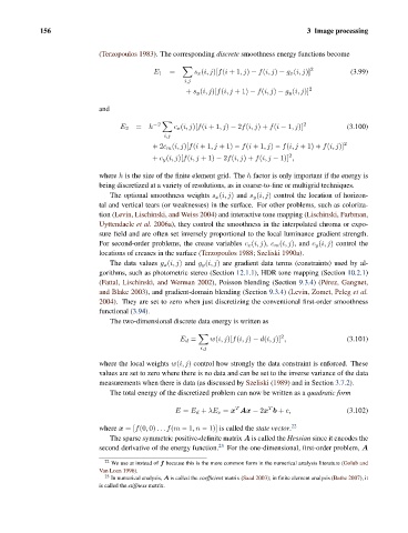
(Terzopoulos 1983). The corresponding discrete smoothness energy functions become

2
= s x (i, j)[f(i +1,j) − f(i, j) − g x (i, j)] (3.99)
E 1
i,j
+ s y (i, j)[f(i, j +1) − f(i, j) − g y (i, j)] 2
and

= h −2 c x (i, j)[f(i +1,j) − 2f(i, j)+ f(i − 1,j)] 2 (3.100)
E 2
i,j
+2c m (i, j)[f(i +1,j +1) − f(i +1,j) − f(i, j +1)+ f(i, j)] 2
2
+ c y (i, j)[f(i, j +1) − 2f(i, j)+ f(i, j − 1)] ,
where h is the size of the finite element grid. The h factor is only important if the energy is
being discretized at a variety of resolutions, as in coarse-to-fine or multigrid techniques.
The optional smoothness weights s x (i, j) and s y (i, j) control the location of horizon-
tal and vertical tears (or weaknesses) in the surface. For other problems, such as coloriza-
tion (Levin, Lischinski, and Weiss 2004) and interactive tone mapping (Lischinski, Farbman,
Uyttendaele et al. 2006a), they control the smoothness in the interpolated chroma or expo-
sure field and are often set inversely proportional to the local luminance gradient strength.
For second-order problems, the crease variables c x (i, j), c m (i, j), and c y (i, j) control the
locations of creases in the surface (Terzopoulos 1988; Szeliski 1990a).
The data values g x (i, j) and g y (i, j) are gradient data terms (constraints) used by al-
gorithms, such as photometric stereo (Section 12.1.1), HDR tone mapping (Section 10.2.1)
(Fattal, Lischinski, and Werman 2002), Poisson blending (Section 9.3.4)(P´ erez, Gangnet,
and Blake 2003), and gradient-domain blending (Section 9.3.4)(Levin, Zomet, Peleg et al.
2004). They are set to zero when just discretizing the conventional first-order smoothness
functional (3.94).
The two-dimensional discrete data energy is written as

2
E d = w(i, j)[f(i, j) − d(i, j)] , (3.101)
i,j
where the local weights w(i, j) control how strongly the data constraint is enforced. These
values are set to zero where there is no data and can be set to the inverse variance of the data
measurements when there is data (as discussed by Szeliski (1989) and in Section 3.7.2).
The total energy of the discretized problem can now be written as a quadratic form

T
T
E = E d + λE s = x Ax − 2x b + c, (3.102)
where x =[f(0, 0) ...f(m − 1,n − 1)] is called the state vector. 22
The sparse symmetric positive-definite matrix A is called the Hessian since it encodes the
second derivative of the energy function. 23 For the one-dimensional, first-order problem, A

22
We use x instead of f because this is the more common form in the numerical analysis literature (Golub and
Van Loan 1996).
23 In numerical analysis, A is called the coefficient matrix (Saad 2003); in finite element analysis (Bathe 2007), it
is called the stiffness matrix.