Page 207 -

186 4 Feature detection and matching

x x i
u

x +u
i i

(a) (b) (c)
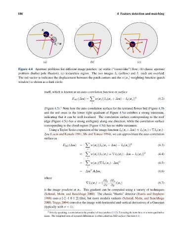
Figure 4.4 Aperture problems for different image patches: (a) stable (“corner-like”) flow; (b) classic aperture
problem (barber-pole illusion); (c) textureless region. The two images I 0 (yellow) and I 1 (red) are overlaid.
The red vector u indicates the displacement between the patch centers and the w(x i ) weighting function (patch
window) is shown as a dark circle.

itself, which is known as an auto-correlation function or surface

E AC (Δu)= w(x i )[I 0 (x i +Δu) − I 0 (x i )] 2 (4.2)
i
1
(Figure 4.5). Note how the auto-correlation surface for the textured flower bed (Figure 4.5b
and the red cross in the lower right quadrant of Figure 4.5a) exhibits a strong minimum,
indicating that it can be well localized. The correlation surface corresponding to the roof
edge (Figure 4.5c) has a strong ambiguity along one direction, while the correlation surface
corresponding to the cloud region (Figure 4.5d) has no stable minimum.
Using a Taylor Series expansion of the image function I 0 (x i +Δu) ≈ I 0 (x i )+∇I 0 (x i )·
Δu (Lucas and Kanade 1981; Shi and Tomasi 1994), we can approximate the auto-correlation
surface as
2
E AC (Δu)= w(x i )[I 0 (x i +Δu) − I 0 (x i )] (4.3)
i
2
≈ w(x i )[I 0 (x i )+ ∇I 0 (x i ) · Δu − I 0 (x i )] (4.4)
i

= w(x i )[∇I 0 (x i ) · Δu] 2 (4.5)
i
T
=Δu AΔu, (4.6)
where
∂I 0 ∂I 0
∇I 0 (x i )=( , )(x i ) (4.7)
∂x ∂y
is the image gradient at x i . This gradient can be computed using a variety of techniques
(Schmid, Mohr, and Bauckhage 2000). The classic “Harris” detector (Harris and Stephens
1988)usesa[-2 -1012] filter, but more modern variants (Schmid, Mohr, and Bauckhage
2000; Triggs 2004) convolve the image with horizontal and vertical derivatives of a Gaussian
(typically with σ =1).

1 Strictly speaking, a correlation is the product of two patches (3.12); I’m using the term here in a more qualitative
sense. The weighted sum of squared differences is often called an SSD surface (Section 8.1).