Page 210 -

4.1 Points and patches 189

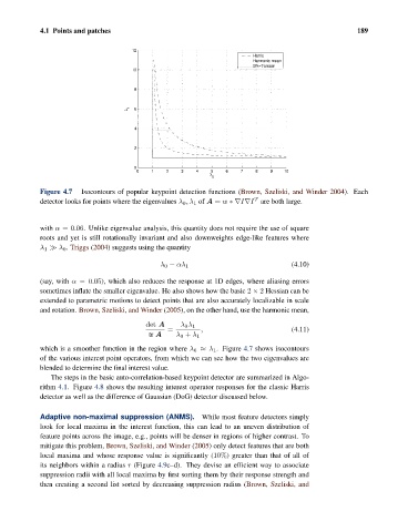
Figure 4.7 Isocontours of popular keypoint detection functions (Brown, Szeliski, and Winder 2004). Each
T
detector looks for points where the eigenvalues λ 0 ,λ 1 of A = w ∗∇I∇I are both large.

with α =0.06. Unlike eigenvalue analysis, this quantity does not require the use of square
roots and yet is still rotationally invariant and also downweights edge-like features where
λ 1 λ 0 . Triggs (2004) suggests using the quantity

(4.10)
λ 0 − αð 1
(say, with α =0.05), which also reduces the response at 1D edges, where aliasing errors
sometimes inflate the smaller eigenvalue. He also shows how the basic 2 × 2 Hessian can be
extended to parametric motions to detect points that are also accurately localizable in scale
and rotation. Brown, Szeliski, and Winder (2005), on the other hand, use the harmonic mean,
det A λ 0 λ 1
= , (4.11)
tr A λ 0 + λ 1

which is a smoother function in the region where λ 0 ≈ λ 1 . Figure 4.7 shows isocontours
of the various interest point operators, from which we can see how the two eigenvalues are
blended to determine the final interest value.
The steps in the basic auto-correlation-based keypoint detector are summarized in Algo-
rithm 4.1. Figure 4.8 shows the resulting interest operator responses for the classic Harris
detector as well as the difference of Gaussian (DoG) detector discussed below.

Adaptive non-maximal suppression (ANMS). While most feature detectors simply
look for local maxima in the interest function, this can lead to an uneven distribution of
feature points across the image, e.g., points will be denser in regions of higher contrast. To
mitigate this problem, Brown, Szeliski, and Winder (2005) only detect features that are both
local maxima and whose response value is significantly (10%) greater than that of all of
its neighbors within a radius r (Figure 4.9c–d). They devise an efficient way to associate
suppression radii with all local maxima by first sorting them by their response strength and
then creating a second list sorted by decreasing suppression radius (Brown, Szeliski, and