Page 211 -

190 4 Feature detection and matching

1. Compute the horizontal and vertical derivatives of the image I x and I y by con-
volving the original image with derivatives of Gaussians (Section 3.2.3).
2. Compute the three images corresponding to the outer products of these gradients.
(The matrix A is symmetric, so only three entries are needed.)

3. Convolve each of these images with a larger Gaussian.

4. Compute a scalar interest measure using one of the formulas discussed above.
5. Find local maxima above a certain threshold and report them as detected feature
point locations.

Algorithm 4.1 Outline of a basic feature detection algorithm.

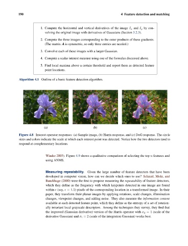
(a) (b) (c)

Figure 4.8 Interest operator responses: (a) Sample image, (b) Harris response, and (c) DoG response. The circle
sizes and colors indicate the scale at which each interest point was detected. Notice how the two detectors tend to
respond at complementary locations.

Winder 2005). Figure 4.9 shows a qualitative comparison of selecting the top n features and
using ANMS.

Measuring repeatability. Given the large number of feature detectors that have been
developed in computer vision, how can we decide which ones to use? Schmid, Mohr, and
Bauckhage (2000) were the first to propose measuring the repeatability of feature detectors,
which they define as the frequency with which keypoints detected in one image are found
within (say, =1.5) pixels of the corresponding location in a transformed image. In their
paper, they transform their planar images by applying rotations, scale changes, illumination
changes, viewpoint changes, and adding noise. They also measure the information content
available at each detected feature point, which they define as the entropy of a set of rotation-
ally invariant local grayscale descriptors. Among the techniques they survey, they find that
the improved (Gaussian derivative) version of the Harris operator with σ d =1 (scale of the
derivative Gaussian) and σ i =2 (scale of the integration Gaussian) works best.