Page 218 -

4.1 Points and patches 197

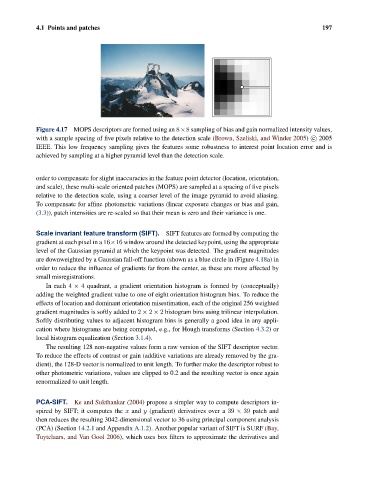
Figure 4.17 MOPS descriptors are formed using an 8×8 sampling of bias and gain normalized intensity values,
with a sample spacing of five pixels relative to the detection scale (Brown, Szeliski, and Winder 2005) c 2005
IEEE. This low frequency sampling gives the features some robustness to interest point location error and is
achieved by sampling at a higher pyramid level than the detection scale.

order to compensate for slight inaccuracies in the feature point detector (location, orientation,
and scale), these multi-scale oriented patches (MOPS) are sampled at a spacing of five pixels
relative to the detection scale, using a coarser level of the image pyramid to avoid aliasing.
To compensate for affine photometric variations (linear exposure changes or bias and gain,
(3.3)), patch intensities are re-scaled so that their mean is zero and their variance is one.

Scale invariant feature transform (SIFT). SIFT features are formed by computing the
gradient at each pixel in a 16×16 window around the detected keypoint, using the appropriate
level of the Gaussian pyramid at which the keypoint was detected. The gradient magnitudes
are downweighted by a Gaussian fall-off function (shown as a blue circle in (Figure 4.18a) in
order to reduce the influence of gradients far from the center, as these are more affected by
small misregistrations.
In each 4 × 4 quadrant, a gradient orientation histogram is formed by (conceptually)
adding the weighted gradient value to one of eight orientation histogram bins. To reduce the
effects of location and dominant orientation misestimation, each of the original 256 weighted
gradient magnitudes is softly added to 2 × 2 × 2 histogram bins using trilinear interpolation.
Softly distributing values to adjacent histogram bins is generally a good idea in any appli-
cation where histograms are being computed, e.g., for Hough transforms (Section 4.3.2)or
local histogram equalization (Section 3.1.4).
The resulting 128 non-negative values form a raw version of the SIFT descriptor vector.
To reduce the effects of contrast or gain (additive variations are already removed by the gra-
dient), the 128-D vector is normalized to unit length. To further make the descriptor robust to
other photometric variations, values are clipped to 0.2 and the resulting vector is once again
renormalized to unit length.

PCA-SIFT. Ke and Sukthankar (2004) propose a simpler way to compute descriptors in-
spired by SIFT; it computes the x and y (gradient) derivatives over a 39 × 39 patch and
then reduces the resulting 3042-dimensional vector to 36 using principal component analysis
(PCA) (Section 14.2.1 and Appendix A.1.2). Another popular variant of SIFT is SURF (Bay,
Tuytelaars, and Van Gool 2006), which uses box filters to approximate the derivatives and