Page 227 -

206 4 Feature detection and matching

(a) (b)
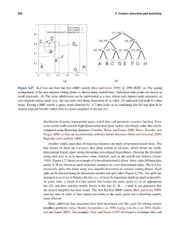
Figure 4.27 K-d tree and best bin first (BBF) search (Beis and Lowe 1999) c 1999 IEEE: (a) The spatial
arrangement of the axis-aligned cutting planes is shown using dashed lines. Individual data points are shown as
small diamonds. (b) The same subdivision can be represented as a tree, where each interior node represents an
axis-aligned cutting plane (e.g., the top node cuts along dimension d1 at value .34) and each leaf node is a data
point. During a BBF search, a query point (denoted by “+”) first looks in its containing bin (D) and then in its
nearest adjacent bin (B), rather than its closest neighbor in the tree (C).

distribution of points in parameter space, which they call parameter-sensitive hashing.Even
more recent work converts high-dimensional descriptor vectors into binary codes that can be
compared using Hamming distances (Torralba, Weiss, and Fergus 2008; Weiss, Torralba, and
Fergus 2008) or that can accommodate arbitrary kernel functions (Kulis and Grauman 2009;
Raginsky and Lazebnik 2009).
Another widely used class of indexing structures are multi-dimensional search trees. The
best known of these are k-d trees, also often written as kd-trees, which divide the multi-
dimensional feature space along alternating axis-aligned hyperplanes, choosing the threshold
along each axis so as to maximize some criterion, such as the search tree balance (Samet
1989). Figure 4.27 shows an example of a two-dimensional k-d tree. Here, eight different data
points A–H are shown as small diamonds arranged on a two-dimensional plane. The k-d tree
recursively splits this plane along axis-aligned (horizontal or vertical) cutting planes. Each
split can be denoted using the dimension number and split value (Figure 4.27b). The splits are
arranged so as to try to balance the tree, i.e., to keep its maximum depth as small as possible.
At query time, a classic k-d tree search first locates the query point (+) in its appropriate
bin (D), and then searches nearby leaves in the tree (C, B, ...) until it can guarantee that
the nearest neighbor has been found. The best bin first (BBF) search (Beis and Lowe 1999)
searches bins in order of their spatial proximity to the query point and is therefore usually
more efficient.

Many additional data structures have been developed over the years for solving nearest
neighbor problems (Arya, Mount, Netanyahu et al. 1998; Liang, Liu, Xu et al. 2001; Hjalta-
son and Samet 2003). For example, Nene and Nayar (1997) developed a technique they call